Missing Data is an interesting data imperfection since it could arise naturally resulting from the character of the domain, or be inadvertently created during data, collection, transmission, or processing.

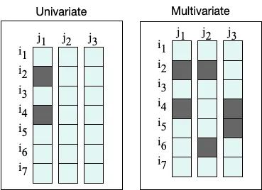
In essence, missing data is characterised by the looks of absent values in data, i.e., missing values in some records or observations within the dataset, and may either be univariate (one feature has missing values) or multivariate (several features have missing values):

Let’s consider an example. Let’s say we’re conducting a study on a patient cohort regarding diabetes, for example.

Medical data is an amazing example for this, since it is usually highly subjected to missing values: patient values are taken from each surveys and laboratory results, will be measured several times throughout the course of diagnosis or treatment, are stored in several formats (sometimes distributed across institutions), and are sometimes handled by different people. It will probably (and most actually will) get messy!

In our diabetes study, a the presence of missing values is perhaps related to the study being conducted or the information being collected.

As an illustration, missing data may arise resulting from a faulty sensor that shuts down for top values of blood pressure. One other possibility is that missing values in feature “weight” usually tend to be missing for older women, that are less inclined to disclose this information. Or obese patients could also be less more likely to share their weight.

However, data may also be missing for reasons which can be on no account related to the study.

A patient can have a few of his information missing because a flat tire caused him to miss a doctors appointment. Data can also be missing resulting from human error: for example, if the person conducting the evaluation misplaces of misreads some documents.

No matter the explanation why data is missing, it can be crucial to research whether the datasets contain missing data prior to model constructing, as this problem can have severe consequences for classifiers:

• Some classifiers cannot handle missing values internally: This makes them inapplicable when handling datasets with missing data. In some scenarios, these values are encoded with a pre-defined value, e.g., “0” in order that machine learning algorithms are capable of deal with them, although this just isn’t the most effective practice, especially for higher percentages of missing data (or more complex missing mechanisms);
• Predictions based on missing data will be biased and unreliable: Although some classifiers can handle missing data internally, their predictions is perhaps compromised, since a crucial piece of knowledge is perhaps missing from the training data.

Furthermore, although missing values may “all look the identical”, the reality is that their underlying mechanisms (that reason why they’re missing) can follow 3 fundamental patters: Missing Completely At Random (MCAR), Missing Not At Random (MNAR), and Missing Not At Random (MNAR).

Keeping these various kinds of missing mechanisms in mind is very important because they determine the selection for appropriate methods to handle missing data efficiently and the validity of the inferences derived from them.

Let’s go over each mechanism real quick!

Missing Data Mechanisms

For those who’re a mathy person, I’d suggest a pass through this paper (cof cof), namely Sections II and III, which comprises all of the notation and mathematical formulation you is perhaps searching for (I used to be actually inspired by this book, which can be a really interesting primer, check Section 2.2.3. and a couple of.2.4.).

For those who’re also a visible learner like me, you’d wish to “see” it, right?

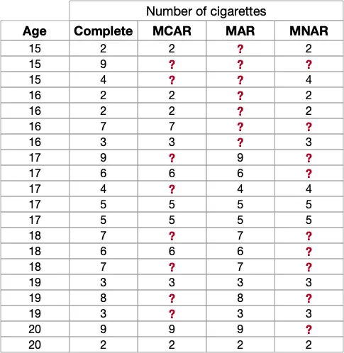
For that matter, we’ll take a take a look at the adolescent tobacco study example, utilized in the paper. We’ll consider dummy data to showcase each missing mechanism:

One thing to take into accout this: the missing mechanisms describe whether and the way the missingness pattern will be explained by the observed data and/or the missing data. It’s tricky, I do know. But it’s going to get more clear with the instance!

In our tobacco study, we’re specializing in adolescent tobacco use. There are 20 observations, relative to twenty participants, and have Age is totally observed, whereas the Variety of Cigarettes (smoked per day) will probably be missing in line with different mechanisms.

Missing Completely At Random (MCAR): No harm, no foul!

In Missing Completely At Random (MCAR) mechanism, the missingness process is totally unrelated to each the observed and missing data. That implies that the probability that a feature has missing values is completely random.

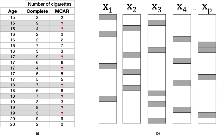
In our example, I simply removed some values randomly. Note how the missing values should not situated in a specific range of Ageor Variety of Cigaretters values. This mechanism can subsequently occur resulting from unexpected events happening through the study: say, the person chargeable for registering the participants’ responses unintentionally skipped a matter of the survey.

Missing At Random (MAR): Search for the tell-tale signs!

The name is definitely misleading, for the reason that Missing At Random (MAR) occurs when the missingness process will be linked to the observed information in data (though to not the missing information itself).

Consider the following example, where I removed the values of Variety of Cigarettes for younger participants only (between 15 and 16 years). Note that, despite the missingess process being clearly related to the observed values in Age, it is totally unrelated to the variety of cigarettes smoked by these teens, had it been reported (note the “Complete” column, where a high and low variety of cigarettes can be found among the many missing values, had they been observed).

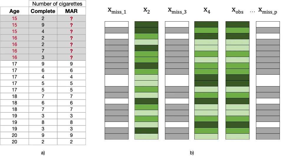
This is able to be the case if younger kids can be less inclined to disclose their variety of smoked cigarettes per day, avoiding to confess that they’re regular smokers (whatever the amount they smoke).

Missing Not At Random (MNAR): That ah-ha moment!

As expected, the Missing Not At Random (MNAR) mechanism is the trickiest of all of them, since the missingness process may depend upon each the observed and missing information in the information. Because of this the probability of missing values occurring in a feature could also be related to the observed values of other feature in the information, in addition to to the missing values of that feature itself!

Take a take a look at the following example: values are missing for higher amounts of Variety of Cigarettes, which suggests that the probability of missing values in Variety of Cigarettes is said to the missing values themselves, had they been observed (note the “Complete” column).

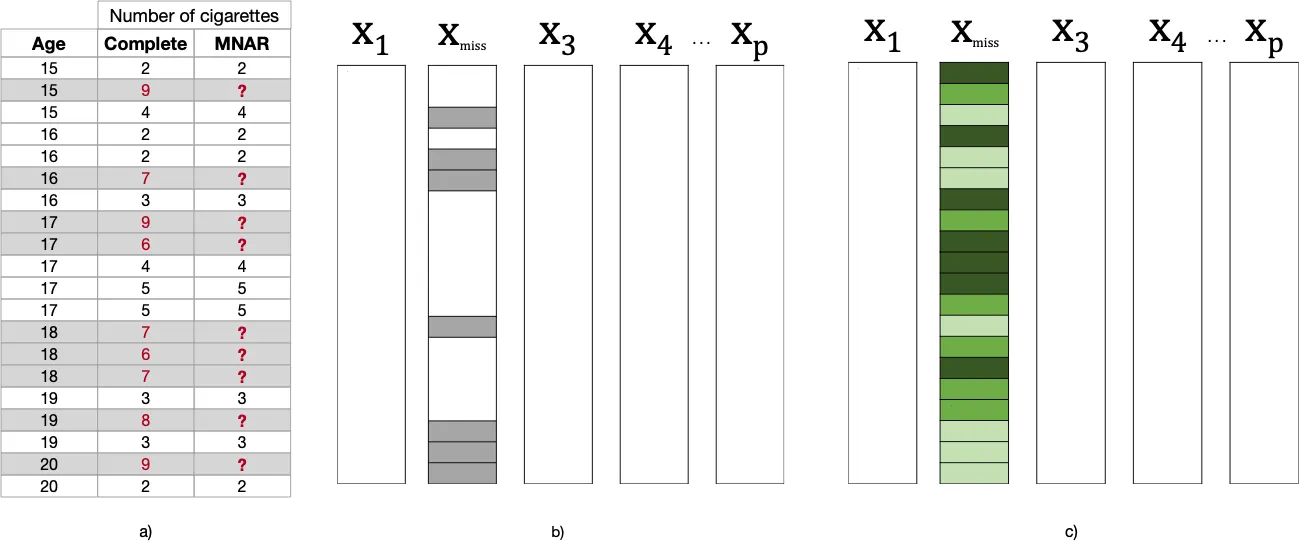
This is able to be the case of teens that refused to report their variety of smoked cigarettes per day since they smoked a really great quantity.

Along our easy example, we’ve seen how MCAR is the best of the missing mechanisms. In such scenario, we may ignore lots of the complexities that arise resulting from the looks of missing values, and some easy fixes akin to case listwise or casewise deletion, in addition to simpler statistical imputation techniques, may do the trick.

Nonetheless, although convenient, the reality is that in real-world domains, MCAR is usually unrealistic, and most researchers normally assume at the least MAR of their studies, which is more general and realistic than MCAR. On this scenario, we may consider more robust strategies than can infer the missing information from the observed data. On this regard, data imputation strategies based on machine learning are generally the most well-liked.

Finally, MNAR is by far essentially the most complex case, since it is vitally difficult to infer the causes for the missingess. Current approaches concentrate on mapping the causes for the missing values using correction aspects defined by domain experts, inferring missing data from distributed systems, extending state-of-the-art models (e.g., generative models) to include multiple imputation, or performing sensitivity evaluation to find out how results change under different circumstances.

Also, on the subject of identifiability, the issue doesn’t get any easier.

Although there are some tests to differentiate MCAR from MAR, they should not widely popular and have restrictive assumptions that don’t hold for complex, real-world datasets. It is usually impossible to differentiate MNAR from MAR for the reason that information that might be needed is missing.

To diagnose and distinguish missing mechanisms in practice, we may concentrate on hypothesis testing, sensitivity evaluation, getting some insights from domain experts, and investigating vizualization techniques that may provide some understanding of the domains.

Naturally, there are other complexities to account for which condition the applying of treatment strategies for missing data, namely the percentage of information that’s missing, the variety of features it affects, and the end goal of the technique (e.g., feed a training model for classification or regression, reconstruct the unique values in essentially the most authentic way possible?).

All in all, not a straightforward job.

Let’s take this little by little. We’ve just learned an overload of knowledge on missing data and its complex entanglements.

In this instance, we’ll cover the fundamentals of the right way to mark and visualize missing data in a real-world dataset, and make sure the issues that missing data introduces to data science projects.

For that purpose, we’ll use the Pima Indians Diabetes dataset, available on Kaggle (License — CC0: Public Domain). For those who’d wish to follow along the tutorial, be at liberty to download the notebook from the Data-Centric AI Community GitHub repository.

To make a fast profiling of your data, we’ll also use ydata-profiling, that gets us a full overview of our dataset in only a couple of line of codes. Let’s start by installing it:

Now, we will load the information and make a fast profile:

Taking a look at the information, we will determine that this dataset consists by 768 records/rows/observations (768 patients), and 9 attributes or features. Actually, End result is the goal class (1/0), so now we have 8 predictors (8 numerical features and 1 categorical).

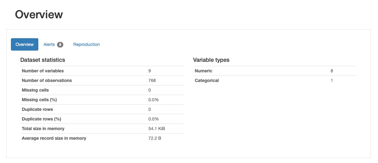
At a primary glance, the dataset doesn’t appear to have missing data. Nonetheless, this dataset is understood to be affected by missing data! How can we confirm that?

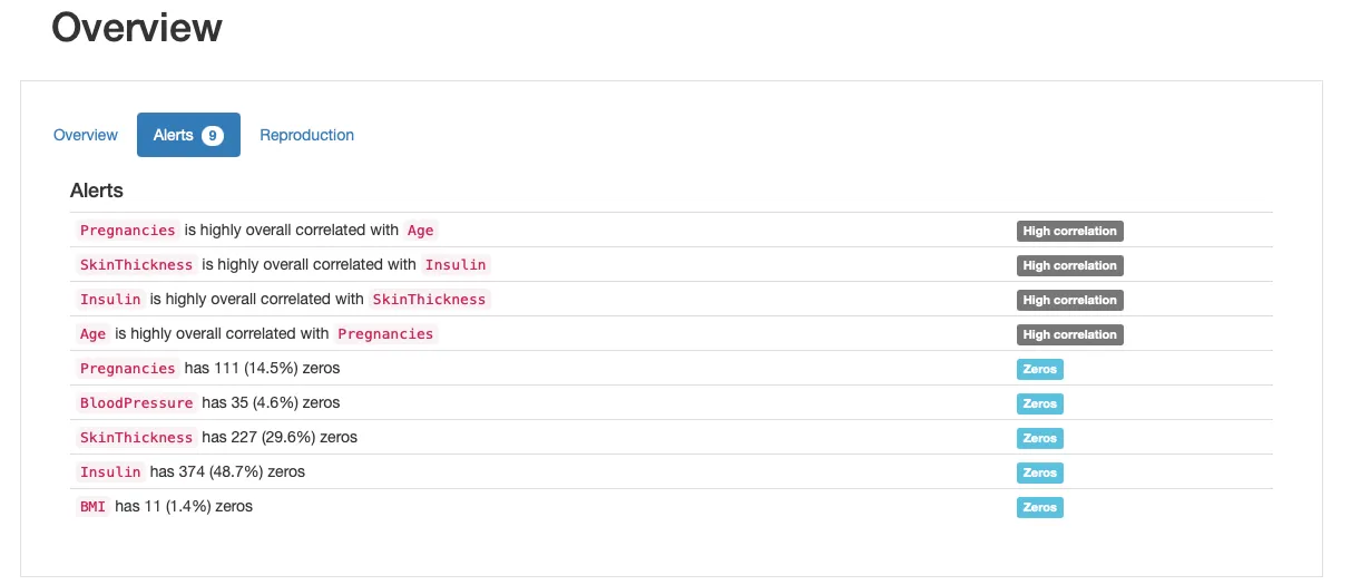
Taking a look at the “Alerts” section, we will see several “Zeros” alerts that indicate us that there are several features for which zero values make no sense or are biologically inconceivable: e.g., a zero-value for body mass index or blood pressure is invalid!

Skimming through all features, we will determine that pregnancies seems fantastic (have zero pregnancies is affordable), but for the remaining features, zero values are suspicious:

In most real-world datasets, missing data is encoded by sentinel values:

• Out-of-range entries, akin to 999;
• Negative numbers where the feature has only positive values, e.g. -1;
• Zero-values in a feature that would never be 0.

In our case, Glucose, BloodPressure, SkinThickness, Insulin, and BMI all have missing data. Let’s count the variety of zeros that these features have:

We will see that Glucose, BloodPressure and BMI have just a couple of zero values, whereas SkinThickness and Insulin have loads more, covering nearly half of the prevailing observations. This implies we would consider different strategies to handle these features: some might require more complex imputation techniques than others, for example.

To make our dataset consistent with data-specific conventions, we should always make these missing values as NaN values.

That is the usual approach to treat missing data in python and the convention followed by popular packages like pandas and scikit-learn. These values are ignored from certain computations like sum or count, and are recognized by some functions to perform other operations (e.g., drop the missing values, impute them, replace them with a set value, etc).

We’ll mark our missing values using the replace() function, after which calling isnan() to confirm in the event that they were appropriately encoded:

The count of NaN values is similar because the 0 values, which suggests that now we have marked our missing values appropriately! We could then use the profile report agains to envision that now the missing data is recognized. Here’s how our “recent” data looks like:

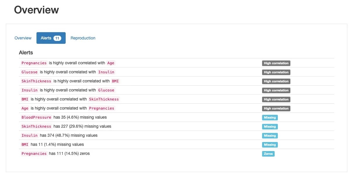
We will further check for some characteristics of the missingness process, skimming through the “Missing Values” section of the report:

Besided the “Count” plot, that provides us an summary of all missing values per feature, we will explore the “Matrix” and “Heatmap” plots in additional detail to hypothesize on the underlying missing mechanisms the information may suffer from. Specifically, the correlation between missing features is perhaps informative. On this case, there appears to be a major correlation between Insulin and SkinThicknes : each values appear to be concurrently missing for some patients. Whether it is a coincidence (unlikely), or the missingness process will be explained by known aspects, namely portraying MAR or MNAR mechanisms can be something for us to dive our noses into!

Regardless, now now we have our data ready for evaluation! Unfortunately, the strategy of handling missing data is removed from being over. Many classic machine learning algorithms cannot handle missing data, and we’d like find expert ways to mitigate the problem. Let’s try to judge the Linear Discriminant Evaluation (LDA) algorithm on this dataset:

For those who attempt to run this code, it’s going to immediately throw an error:

The only approach to fix this (and essentially the most naive!) can be to remove all records that contain missing values. We will do that by making a recent data frame with the rows containing missing values removed, using the dropna() function…

… and trying again:

And there you’ve gotten it! By the dropping the missing values, the LDA algorithm can now operate normally.

Nonetheless, the dataset size was substantially reduced to 392 observations only, which suggests we’re losing nearly half of the available information.

For that reason, as an alternative of simply dropping observations, we should always search for imputation strategies, either statistical or machine-learning based. We could also use synthetic data to exchange the missing values, depending on our final application.

And for that, we would attempt to get some insight on the underlying missing mechanisms in the information. Something to stay up for in future articles?