Kernel Case Study: Flash Attention

mechanism is on the core of recent day transformers. But scaling the context window of those transformers was a significant challenge, and it still is despite the fact that we’re within the era of 1,000,000 tokens + context window (Qwen 2.5 [1]). There are each considerable compute and memory sure complexities in these models after we scale the context window (A naive Attention Mechanism scales quadratically in each compute and memory requirements). Revisiting Flash Attention lets us understand the complexities of optimizing the underlying operations on GPUs and more importantly gives us a greater grip on considering what’s next.

Let’s quickly revisit a naive attention algorithm to see what’s happening.

As you’ll be able to see if we should not being careful then we’ll find yourself materializing a full NxM attention matrix into the GPU HBM. Meaning the memory requirement will go up quadratically to increasing context length.

For those who wanna learn more concerning the GPU memory hierarchy and its differences, my previous post on Triton is a very good place to begin. This might even be handy as we go along on this post after we get to implementing the Flash Attention kernel in triton. The flash attention paper also has some really good introduction to this.

Moreover, after we take a look at the steps involved in executing this algorithm and its pattern of accessing the slow HBM, (which as explained later within the post may very well be a significant bottleneck as well) we notice a couple of things:

1. We have now Q, K and V within the HBM initially
2. We want to access Q and K initially from the HBM to compute the dot product
3. We write the output scores back to the HBM
4. We access it again to execute the softmax, and optionally for Causal attention, like within the case of LLMs, we could have to mask this output before the softmax. The resulting full attention matrix is written again into the HBM
5. We access the HBM again to execute the ultimate dot product, to get each the eye weights and the Value matrix to write down the output back to the slow GPU memory

I feel you get the purpose. We could smartly read and write from the HBM to avoid redundant operations, to make some potential gains. This is precisely the first motivation for the unique Flash Attention algorithm.

Flash Attention initially got here out in 2022 [2], after which a yr later got here out with some much needed improvements in 2023 as Flash Attention v2 [3] and again in 2024 with additional improvements for Nvidia Hopper and Blackwell GPUs [4] as Flash Attention v3 [5]. The unique attention paper identified that the eye operation remains to be limited by memory bandwidth moderately than compute. (Prior to now, there have been attempts to cut back the computation complexity of Attention from O(N**2) to O(NlogN) and lower through approximate algorithms)

Flash attention proposed a fused kernel which does all the above attention operations in a single go, block-wise, to get the ultimate attention output without ever having to appreciate the complete N**2 attention matrix in memory, making the algorithm significantly faster. The term `fused` simply means we mix multiple operations within the GPU SRAM before invoking the much slower journey across the slower GPU memory, making the algorithm performant. All of the while providing the precise attention output with none approximations.

This lecture, from Stanford CS139, demonstrates brilliantly how we are able to consider the impact of a well thought out memory access pattern can have on an algorithm. I highly recommend you check this one out in case you haven’t already.

Before we start diving into flash attention to call it FA, lets?) in triton there’s something else that I desired to get out of the best way.

Numerical Stability in exponents

Let’s take the instance of FP32 numbers. float32 (standard 32-bit float) uses 1 sign bit, 8 exponent bits, and 23 mantissa bits [6]. The biggest finite base for the exponent in float32 is 2¹²⁷≈1.7×10³⁸. Which suggests after we take a look at exponents, e⁸⁸ ≈ 1.65×10³⁸, anything near 88 (although in point of fact can be much lower to maintain it protected) and we’re in trouble as we could easily overflow. Here’s a very interesting chat with OpenAI o1 shared by folks at AllenAI of their OpenInstruct repo. This although is talking about stabilizing KL Divergence calculations within the setting of RLHF/RL, the ideas translate exactly to exponents as well. So to take care of the softmax situation in attention what we do is the next:

TRICK : Let’s also observe the next, in case you do that:

then you definately can rescale/readjust values without affecting the ultimate softmax value. This is admittedly useful when you have got an initial estimate for the utmost value, but which may change after we encounter a brand new set of values. I do know I do know, stick with me and let me explain.

Setting the scene

Let’s take a small detour into matrix multiplication.

This shows a toy example of a blocked matrix multiplication except we have now blocks only on the rows of A (green) and columns of B (Orange? Beige?). As you’ll be able to see above the output O1, O2, O3 and O4 are complete (those positions need no more calculations). We just must fill within the remaining columns within the initial rows by utilizing the remaining columns of B. Like below:

So we are able to fill these places within the output with a block of columns from B and a block of rows from A at a time.

Connecting the dots

Once I introduced FA, I said that we never should compute the complete attention matrix and store the entire thing. So here’s what we do:

1. Compute a block of the eye matrix using a block of rows from Q and a block of columns from K. When you get the partial attention matrix compute a couple of statistics and keep it within the memory.

I even have greyed O5 to O12 because we don’t know those values yet, as they need to return from the next blocks. We then transform Sb like below:

Now you have got setup for a partial softmax

But:

1. What if the true maximum is within the Oi’s which are yet to return?
2. The sum remains to be local, so we’d like to update this each time we see latest Pi’s. We all know tips on how to keep track of a sum, but what about rebasing it to the true maximum?

Recall the trick above. All that we have now to do is to maintain a track of the utmost values we encounter for every row, and iteratively update as you see latest maximums from the remaining blocks of columns from K for a similar set of rows from Q.

We still don’t need to write down our partial softmax matrix into HBM. We keep it for the subsequent step.

The ultimate dot product

The last step in our attention computation is our dot product with V. To begin we’d have initialized a matrix filled with 0’s in our HBM as our output of shape NxD. Where N is the variety of Queries as above. We use the identical block size for V as we had for K except we are able to apply it row clever like below (The subscripts just denote that this is barely a block and never the complete matrix)

Notice how we’d like the eye scores from all of the blocks to get the ultimate product. But when we calculate the local rating and `accumulate` it like how we did to get the actual Ls we are able to form the complete output at the top of processing all of the blocks of columns (K_b) for a given row block (Q_b).

Putting all of it together

Let’s put all these ideas together to form the ultimate algorithm

To know the notation, __ij implies that it’s the local values for a given block of columns and rows and _i implies it’s for the worldwide output rows and Query blocks. The one part we haven’t explained to date is the ultimate update to O_i. That’s where we use all of the ideas from above to get the precise scaling.

The entire code is offered as a gist here.

Let’s see what these initializations appear like in torch:

def flash_attn_v1(Q, K, V, Br, Bc):
  """Flash Attention V1"""
  B, N, D = Q.shape
  M = K.shape[1]
  Nr = int(np.ceil(N/Br))
  Nc = int(np.ceil(N/Bc))
  
  Q = Q.to('cuda')
  K = K.to('cuda')
  V = V.to('cuda')
  
  batch_stride = Q.stride(0)
  
  O = torch.zeros_like(Q).to('cuda')
  lis = torch.zeros((B, Nr, int(Br)), dtype=torch.float32).to('cuda')
  mis = torch.ones((B, Nr, int(Br)), dtype=torch.float32).to('cuda')*-torch.inf
  
  grid = (B, )
  flash_attn_v1_kernel[grid](
      Q, K, V,
      N, M, D,
      Br, Bc,
      Nr, Nc,
      batch_stride,
      Q.stride(1),
      K.stride(1),
      V.stride(1),
      lis, mis,
      O,
      O.stride(1),
  )
  return O

For those who are unsure concerning the launch grid, checkout my introduction to Triton

Take a more in-depth take a look at how we initialized our Ls and Ms. We’re keeping one for every row block of Output/Query, each of size B_r. There are N_r such blocks in total.

In the instance above I used to be simply using B_r = 2 and B_c = 2. But within the above code the initialization is predicated on the device capability. I even have included the calculation for a T4 GPU. For another GPU, we’d like to get the SRAM capability and adjust these numbers accordingly. Now for the actual kernel implementation:

# Flash Attention V1
import triton
import triton.language as tl
import torch
import numpy as np
import pdb

@triton.jit
def flash_attn_v1_kernel(
    Q, K, V,
    N: tl.constexpr, M: tl.constexpr, D: tl.constexpr,
    Br: tl.constexpr,
    Bc: tl.constexpr,
    Nr: tl.constexpr,
    Nc: tl.constexpr,
    batch_stride: tl.constexpr,
    q_rstride: tl.constexpr,
    k_rstride: tl.constexpr, 
    v_rstride: tl.constexpr,
    lis, mis,
    O,
    o_rstride: tl.constexpr):
    
    """Flash Attention V1 kernel"""
    
    pid = tl.program_id(0)
    

    for j in range(Nc):
        k_offset = ((tl.arange(0, Bc) + j*Bc) * k_rstride)[:, None] + (tl.arange(0, D))[None, :] + pid * M * D
        # Using k_rstride and v_rstride as we're  your complete row directly, for every k v block 
        v_offset = ((tl.arange(0, Bc) + j*Bc) * v_rstride)[:, None] + (tl.arange(0, D))[None, :] + pid * M * D
        k_mask = k_offset < (pid + 1) * M*D
        v_mask = v_offset < (pid + 1) * M*D
        k_load = tl.load(K + k_offset, mask=k_mask, other=0)
        v_load = tl.load(V + v_offset, mask=v_mask, other=0)
        for i in range(Nr):
            q_offset = ((tl.arange(0, Br) + i*Br) * q_rstride)[:, None] + (tl.arange(0, D))[None, :] + pid * N * D
            q_mask = q_offset < (pid + 1) * N*D
            q_load = tl.load(Q + q_offset, mask=q_mask, other=0)
            # Compute attention
            s_ij = tl.dot(q_load, tl.trans(k_load))
            m_ij = tl.max(s_ij, axis=1, keep_dims=True)
            p_ij = tl.exp(s_ij - m_ij)
            l_ij = tl.sum(p_ij, axis=1, keep_dims=True)
            
            ml_offset = tl.arange(0, Br) + Br * i + pid * Nr * Br
            m = tl.load(mis + ml_offset)[:, None]
            l = tl.load(lis + ml_offset)[:, None]

            m_new = tl.where(m < m_ij, m_ij, m)

            l_new = tl.exp(m - m_new) * l + tl.exp(m_ij - m_new) * l_ij

            o_ij = tl.dot(p_ij, v_load)

            output_offset = ((tl.arange(0, Br) + i*Br) * o_rstride)[:, None] + (tl.arange(0, D))[None, :] + pid * N * D
            output_mask = output_offset < (pid + 1) * N*D
            o_current = tl.load(O + output_offset, mask=output_mask)

            o_new = (1/l_new) * (l * tl.exp(m - m_new) * o_current + tl.exp(m_ij - m_new) * o_ij)

            tl.store(O + output_offset, o_new, mask=output_mask)
            tl.store(mis + ml_offset, tl.reshape(m_new, (Br,)))
            tl.store(lis + ml_offset, tl.reshape(l_new, (Br,)))

Let’s understand whats happening here:

1. Create 1 kernel for every NxD matrix within the batch. In point of fact we'd have yet one more dimension to parallelize across, the top dimension. But for understanding the implementation I feel this may suffice.
2. In each kernel we do the next:
   1. For every block of columns in K and V we load up the relevant a part of the matrix (B_c x D) into the GPU SRAM (Current total SRAM usage = 2B_cD). This stays within the SRAM till we're done with all of the row blocks
   2. For every row block of Q, we load the block onto SRAM as well (Current total SRAM Usage = 2B_cD + BrD)
   3. On chip we compute the dot product (s_ij), compute the local row-maxes (m_ij), the exp (p_ij), and the expsum (l_ij)
   4. We load up the running stats for the i^th row block. Two vectors of size B_r x 1, which denotes the present global row-maxes (m_i) and the expsum (l_i). (Current SRAM usage: 2B_cD + B_rD + 2B_r)
   5. We get the brand new estimates for the worldwide m_i and l_i.
   6. We load the a part of the output for this block of Q and update it using the brand new running stats and the exponent trick, we then write this back into the HBM. (Current SRAM usage: 2B_cD + 2B_rD + 2B_r)
   7. We write the updated running stats also into the HBM.
3. For a matrix of any size, aka any context length, at a time we'll never materialize the complete attention matrix, only an element of it at all times.
4. We managed to fuse together all of the ops right into a single kernel, reducing HBM access considerably.

Final SRAM usage stands although at 4BD + 2B, where B was initially calculated as M/4d where M is the SRAM capability. Unsure if am missing something here. Please comment in case you know why that is the case!

Block Sparse Attention and V2 and V3

I'll keep this short as these versions keep the core idea but found out higher and higher ways to do the identical.

For Block Sparse Attention,

1. Consider we had masks for every block like within the case of causal attention. If for a given block we have now the masks all set to zero then we are able to simply skip your complete block without computing anything really. Saving FLOPs. That is where the foremost gains were seen. To place this into perspective, within the case of BERT pre-training the algorithm gets a 15% boost over the most effective performing training setup on the time, whereas for GPT-2 we get a 3x over huggingface training implementation and ~ 2x over a Megatron setup.

2. You may literally get the identical performance in GPT2 in a fraction of the time, literally shaving off days from the training run, which is awesome!

In V2:

1. Notice how currently we are able to only do parallelization on the batch and head dimension. But in case you simply just flip the order to take a look at all of the column blocks for a given row block then we get the next benefits:
   1. Each row block becomes embarrassingly parallel. How you recognize that is by the illustrations above. You would like all of the column blocks for a given row block to completely form the eye output. For those who were to run all of the column blocks in parallel, you'll find yourself with a race condition that can attempt to update the identical rows of the output at the identical time. But not in case you do it the opposite way around. Although there are atomic add operators in triton which could help, they could potentially set us back.
   2. We are able to avoid hitting the HBM to get the worldwide Ms and Ls. We are able to initialize one on the chip for every kernel.
   3. Also we should not have to scale all of the output update terms with the brand new estimate of L. We are able to just compute stuff without dividing by L and at the top of all of the column blocks, simply divide the output with the newest estimate of L, saving some FLOPS again!
2. Much of the development also is available in the shape of the backward kernel. I'm omitting all of the backward kernels from this. But they're a fun exercise to try to implement, although they're significantly more complex.

Listed here are some benchmarks:

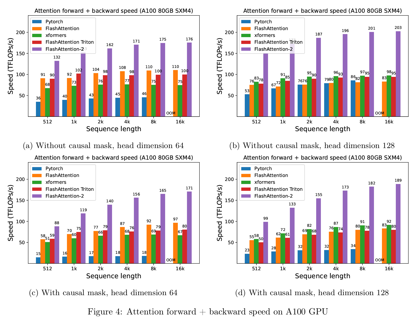
The actual implementations of those kernels must keep in mind various nuances that we encounter in the true world. I even have tried to maintain it easy. But do check them out here.

More recently in V3:

1. Newer GPUs, especially the Hopper and Blackwell GPUs, have low precision modes (FP8 in Hopper and GP4 in Blackwell), which might double and quadruple the throughput for a similar power and chip area and more specialized GEMM (General Matrix Multiply) kernels, which the previous version of the algorithm fails to capitalize on. It is because there are various operations that are non-GEMM, like softmax, which reduces the utilization of those specialized GPU kernels.
2. The FA v1 and v2 are essentially synchronous. Recall within the v2 description I discussed that we're limited when column blocks try to write down to the identical output pointers, or when we have now to go step-by-step using the output from the previous steps. Well these modern GPUs could make use special instructions to interrupt this synchrony.

3. In addition they adapted the algorithm to focus on these specialized low precision Tensor cores on these latest devices, significantly increasing the FLOPs.

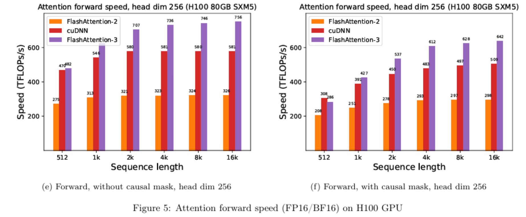
Some more benchmarks:

Conclusion

There may be much to admire of their work here. The ground for this technical skill level often seemed high owing to the low level details. But hopefully tools like Triton could change the sport and get more people into this! The longer term is shiny.

References

[1] Qwen 2.5-7B-Instruct-1M Huggingface Model Page

[2] Re,

[3] Tri Dao,

[4] NVIDIA Hopper Architecture Page

[5] Jay Shah, Ganesh Bikshandi, Ying Zhang, Vijay Thakkar, Pradeep Ramani, Tri Dao, FlashAttention-3: Fast and Accurate Attention with Asynchrony and Low-precision

[6] Single-precision floating-point format, Wikipedia