
Previously we discussed applying reinforcement learning to Extraordinary Differential Equations (ODEs) by integrating ODEs inside gymnasium. ODEs are a strong tool that may describe a wide selection of systems but are limited to a single variable. Partial Differential Equations (PDEs) are differential equations involving derivatives of multiple variables that may cover a far broader range and more complex systems. Often, ODEs are special cases or special assumptions applied to PDEs.
PDEs include Maxwell’s Equations (governing electricity and magnetism), Navier-Stokes equations (governing fluid flow for aircraft, engines, blood, and other cases), and the Boltzman equation for thermodynamics. PDEs can describe systems similar to flexible structures, power grids, manufacturing, or epidemiological models in biology. They will represent highly complex behavior; the Navier Stokes equations describe the eddies of a rushing mountain stream. Their capability for capturing and revealing more complex behavior of real-world systems makes these equations a crucial topic for study, each by way of describing systems and analyzing known equations to make recent discoveries about systems. Entire fields (like fluid dynamics, electrodynamics, structural mechanics) might be devoted to review of only a single set of PDEs.
This increased complexity comes with a price; the systems captured by PDEs are rather more difficult to research and control. ODEs are also described as lumped-parameter systems, the assorted parameters and variables that describe them are “lumped” right into a discrete point (or small variety of points for a coupled system of ODEs). PDEs are distributed parameter systems that track behavior throughout space and time. In other words, the state space for an ODE is a comparatively small variety of variables, similar to time and a couple of system measurements at a selected point. For PDE/distributed parameter systems, the state space size can approach infinite dimensions, or discretized for computation into tens of millions of points . A lumped parameter system controls the temperature of an engine based on a small variety of sensors. A PDE/distributed parameter system would manage temperature dynamics across your complete engine.
As with ODEs, many PDEs have to be analyzed (apart from special cases) through modelling and simulation. Nonetheless, because of the upper dimensions, this modelling becomes way more complex. Many ODEs might be solved through straightforward applications of algorithms like MATLAB’s ODE45 or SciPy’s solve_ivp. PDEs are modelled across grids or meshes where the PDE is simplified to an algebraic equation (similar to through Taylor Series expansion) at each point on the grid. Grid generation is a field, a science and art, by itself and ideal (or usable) grids can vary greatly based on problem geometry and Physics. Grids (and hence problem state spaces) can number within the tens of millions of points with computation time running in days or even weeks, and PDE solvers are sometimes business software costing tens of hundreds of dollars.
Controlling PDEs presents a far greater challenge than ODEs. The Laplace transform that forms the idea of much classical control theory is a one-dimensional transformation. While there was some progress in PDE control theory, the sector isn’t as comprehensive as for ODE/lumped systems. For PDEs, even basic controllability or observability assessments turn out to be difficult because the state space to evaluate increases by orders of magnitude and fewer PDEs have analytic solutions. By necessity, we run into design questions similar to what a part of the domain must be controlled or observed? Can the remaining of the domain be in an arbitrary state? What subset of the domain does the controller must operate over? With key tools on top of things theory underdeveloped, and recent problems presented, applying machine learning has been a serious area of research for understanding and controlling PDE systems.
Given the importance of PDEs, there was research into developing control strategies for them. For instance, Glowinski et. all developed an analytical adjoint based method from advanced functional evaluation counting on simulation of the system. Other approaches, similar to discussed by Kirsten Morris, apply estimations to cut back the order of the PDE to facilitate more traditional control approaches. Botteghi and Fasel, have begun to use machine learning to regulate of those systems (note, this is simply a VERY BRIEF glimpse of the research). Here we’ll apply reinforcement learning on two PDE control problems. The diffusion equation is an easy, linear, second order PDE with known analytic solution. The Kuramoto–Sivashinsky (K-S) equation is a rather more complex 4th order nonlinear equation that models instabilities in a flame front.
For each these equations we use a straightforward, small square domain of grid points. We goal a sinusoidal pattern in a goal area of a line down the center of the domain by controlling input along left and right sides. Input parameters for the controls are the values on the goal region and the {x,y} coordinates of the input control points. Training the algorithm required modelling the system development through time with the control inputs. As discussed above, this requires a grid where the equation is solved at each point then iterated through every time step. I used the py-pde package to create a training environment for the reinforcement learner (due to the developer of this package for his prompt feedback and help!). With the py-pde environment, approach proceeded as usual with reinforcement learning: the actual algorithm develops a guess at a controller strategy. That controller strategy is applied at small, discrete time steps and provides control inputs based on the present state of the system that result in some reward (on this case, root mean square difference between goal and current distribution).
Unlike previous cases, I only present results from the genetic-programming controller. I developed code to use a soft actor critic (SAC) algorithm to execute as a container on AWS Sagemaker. Nonetheless, full execution would take about 50 hours and I didn’t need to spend the cash! I looked for methods to cut back the computation time, but eventually gave up because of time constraints; this text was already taking long enough to get out with my job, military reserve duty, family visits over the vacations, civic and church involvement, and never leaving my wife to maintain our baby boy alone!
First we’ll discuss the diffusion equation:
with x as a two dimensional cartesian vector and ∆ the Laplace operator. As mentioned, this is an easy second order (second derivative) linear partial differential equation in time and two dimensional space. Mu is the diffusion coefficient which determines how briskly effects travel through the system. The diffusion equation tends to wash-out (diffuse!) effects on the boundaries throughout the domain and exhibits stable dynamics. The PDE is implemented as shown below with grid, equation, boundary conditions, initial conditions, and goal distribution:
from pde import Diffusion, CartesianGrid, ScalarField, DiffusionPDE, pde
grid = pde.CartesianGrid([[0, 1], [0, 1]], [20, 20], periodic=[False, True])
state = ScalarField.random_uniform(grid, 0.0, 0.2)
bc_left={"value": 0}
bc_right={"value": 0}
bc_x=[bc_left, bc_right]
bc_y="periodic"
#bc_x="periodic"
eq = DiffusionPDE(diffusivity=.1, bc=[bc_x, bc_y])
solver=pde.ExplicitSolver(eq, scheme="euler", adaptive = True)
#result = eq.solve(state, t_range=dt, adaptive=True, tracker=None)
stepper=solver.make_stepper(state, dt=1e-3)
goal = 1.*np.sin(2*grid.axes_coords[1]*3.14159265)
The issue is sensitive to diffusion coefficient and domain size; mismatch between these two ends in washing out control inputs before they will reach the goal region unless calculated over a protracted simulation time. The control input was updated and reward evaluated every 0.1 timestep as much as an end time of T=15.
Attributable to py-pde package architecture, the control is applied to at least one column contained in the boundary. Structuring the py-pde package to execute with the boundary condition updated every time step resulted in a memory leak, and the py-pde developer advised using a stepper function as a work-around that doesn’t allow updating the boundary condition. This implies the outcomes aren’t exactly physical, but do display the fundamental principle of PDE control with reinforcement learning.
The GP algorithm was capable of arrive at a final reward (sum mean square error of all 20 points within the central column) of about 2.0 after about 30 iterations with a 500 tree forest. The outcomes are shown below as goal and achieved distributed within the goal region.

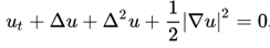
Now the more interesting and sophisticated K-S equation:
Unlike the diffusion equation, the K-S equation displays wealthy dynamics (as befitting an equation describing flame behavior!). Solutions may include stable equilibria or travelling waves, but with increasing domain size all solutions will eventually turn out to be chaotic. The PDE implementation is given by below code:
grid = pde.CartesianGrid([[0, 10], [0, 10]], [20, 20], periodic=[True, True])
state = ScalarField.random_uniform(grid, 0.0, 0.5)
bc_y="periodic"
bc_x="periodic"
eq = PDE({"u": "-gradient_squared(u) / 2 - laplace(u + laplace(u))"}, bc=[bc_x, bc_y])
solver=pde.ExplicitSolver(eq, scheme="euler", adaptive = True)
stepper=solver.make_stepper(state, dt=1e-3)
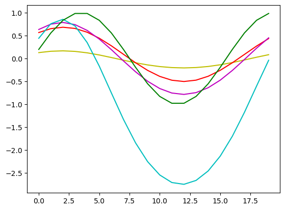
goal=1.*np.sin(0.25*grid.axes_coords[1]*3.14159265)Control inputs are capped at +/-5. The K-S equation is of course unstable; if any point within the domain exceeds +/- 30 the iteration terminates with a big negative reward for causing the system to diverge. Experiments with the K-S equation in py-pde revealed strong sensitivity to domain size and variety of grid points. The equation was run for T=35, each with control and reward update at dt=0.1.
For every, the GP algorithm had more trouble arriving at an answer than within the diffusion equation. I selected to manually stop execution when the answer became visually close; again, we’re in search of general principles here. For the more complex system, the controller works higher—likely due to how dynamic the K-S equation is the controller is capable of have a much bigger impact. Nonetheless, when evaluating the answer for various run times, I discovered it was not stable; the algorithm learned to reach on the goal distribution at a selected time, to not stabilize at that solution. The algorithm converged to the below solution, but, because the successive time steps show, the answer is unstable and begins to diverge with increasing time steps.
Careful tuning on the reward function would help obtain an answer that may hold longer, reinforcing how vital correct reward function is. Also, in all these cases we aren’t coming to perfect solutions; but, especially for the K-S equations we’re getting decent solutions with comparatively little effort in comparison with non-RL approaches for tackling these styles of problems.
The GP solution is taking longer to resolve with more complex problems and has trouble handling large input variable sets. To make use of larger input sets, the equations it generates turn out to be longer which make it less interpretable and slower to compute. Solution equations had scores of terms moderately than the dozen or so in ODE systems. Neural network approaches can handle large input variable sets more easily as input variables only directly impact the dimensions of the input layer. Further, I believe that neural networks will have the opportunity to handle more complex and bigger problems higher for reasons discussed previously in previous posts. Due to that, I did develop gymnasiums for py-pde diffusion, which may easily be adapted to other PDEs per the py-pde documentation. These gymnasiums might be used with different NN-based reinforcement learning similar to the SAC algorithm I developed (which, as discussed, runs but takes time).
Adjustments is also made to the genetic Programming approach. For instance, vector representation of inputs could reduce size of solution equations. Duriez et al.1 all proposes using Laplace transform to introduce derivatives and integrals into the genetic programming equations, broadening the function spaces they will explore.
The flexibility to tackle more complex problems is vital. As discussed above, PDEs can describe a wide selection of complex phenomena. Currently, controlling these systems often means lumping parameters. Doing so leaves out dynamics and so we find yourself working against such systems moderately than with them. Efforts to regulate or manage these means higher control effort, missed efficiencies, and increased risk of failure (small or catastrophic). Higher understanding and control alternatives for PDE systems could unlock major gains in engineering fields where marginal improvements have been the usual similar to traffic, supply chains, and nuclear fusion as these systems behave as high dimensional distributed parameter systems. They’re highly complex with nonlinear and emergent phenomena but have large available data sets—ideal for machine learning to maneuver past current barriers in understanding and optimization.
For now, I even have only taken a really basic have a look at applying ML to controlling PDEs. Follow ons to the control problem include not only different systems, but optimizing where within the domain the control is applied, experimenting with reduced-order statement space, and optimizing the control for simplicity or control effort. Along with improved control efficiency, as discussed in Brunton and Kutz2, machine learning may also be used to derive data-based models of complex physical systems and to find out reduced order models which reduce state space size and will be more amenable to evaluation and control, by traditional or machine learning methods. Machine learning and PDEs is an exciting area of research, and I encourage you to see what the professionals are doing!