Optimizing your LLM in production

Note: This blog post can also be available as a documentation page on Transformers.

Large Language Models (LLMs) resembling GPT3/4, Falcon, and LLama are rapidly advancing of their ability to tackle human-centric tasks, establishing themselves as essential tools in modern knowledge-based industries.
Deploying these models in real-world tasks stays difficult, nevertheless:

• To exhibit near-human text understanding and generation capabilities, LLMs currently require to be composed of billions of parameters (see Kaplan et al, Wei et. al). This consequently amplifies the memory demands for inference.
• In lots of real-world tasks, LLMs have to be given extensive contextual information. This necessitates the model’s capability to administer very long input sequences during inference.

The crux of those challenges lies in augmenting the computational and memory capabilities of LLMs, especially when handling expansive input sequences.

On this blog post, we’ll go over essentially the most effective techniques on the time of writing this blog post to tackle these challenges for efficient LLM deployment:

1. Lower Precision: Research has shown that operating at reduced numerical precision, namely 8-bit and 4-bit, can achieve computational benefits with out a considerable decline in model performance.

2. Flash Attention: Flash Attention is a variation of the eye algorithm that not only provides a more memory-efficient approach but additionally realizes increased efficiency on account of optimized GPU memory utilization.

3. Architectural Innovations: Considering that LLMs are at all times deployed in the identical way during inference, namely autoregressive text generation with a protracted input context, specialized model architectures have been proposed that allow for more efficient inference. Crucial advancement in model architectures hereby are Alibi, Rotary embeddings, Multi-Query Attention (MQA) and Grouped-Query-Attention (GQA).

Throughout this notebook, we’ll offer an evaluation of auto-regressive generation from a tensor’s perspective. We delve into the professionals and cons of adopting lower precision, provide a comprehensive exploration of the most recent attention algorithms, and discuss improved LLM architectures. While doing so, we run practical examples showcasing each of the feature improvements.

1. Harnessing the Power of Lower Precision

Memory requirements of LLMs might be best understood by seeing the LLM as a set of weight matrices and vectors and the text inputs as a sequence of vectors. In the next, the definition weights will probably be used to indicate all model weight matrices and vectors.

On the time of writing this post, LLMs consist of not less than a pair billion parameters. Each parameter thereby is manufactured from a decimal number, e.g. 4.5689 which is often stored in either float32, bfloat16, or float16 format. This permits us to simply compute the memory requirement to load the LLM into memory:

Loading the weights of a model having X billion parameters requires roughly 4 * X GB of VRAM in float32 precision

Nowadays, models are nevertheless rarely trained in full float32 precision, but normally in bfloat16 precision or less regularly in float16 precision. Due to this fact the rule of thumb becomes:

Loading the weights of a model having X billion parameters requires roughly 2 * X GB of VRAM in bfloat16/float16 precision

For shorter text inputs (lower than 1024 tokens), the memory requirement for inference may be very much dominated by the memory requirement to load the weights. Due to this fact, for now, let’s assume that the memory requirement for inference is the same as the memory requirement to load the model into the GPU VRAM.

To present some examples of how much VRAM it roughly takes to load a model in bfloat16:

• GPT3 requires 2 * 175 GB = 350 GB VRAM
• Bloom requires 2 * 176 GB = 352 GB VRAM
• Llama-2-70b requires 2 * 70 GB = 140 GB VRAM
• Falcon-40b requires 2 * 40 GB = 80 GB VRAM
• MPT-30b requires 2 * 30 GB = 60 GB VRAM
• bigcode/starcoder requires 2 * 15.5 = 31 GB VRAM

As of writing this document, the biggest GPU chip available on the market is the A100 offering 80GB of VRAM. A lot of the models listed before require greater than 80GB simply to be loaded and subsequently necessarily require tensor parallelism and/or pipeline parallelism.

🤗 Transformers doesn’t support tensor parallelism out of the box because it requires the model architecture to be written in a particular way. When you’re all for writing models in a tensor-parallelism-friendly way, be happy to have a take a look at the text-generation-inference library.

Naive pipeline parallelism is supported out of the box. For this, simply load the model with device="auto" which can mechanically place different layers on the available GPUs as explained here.
Note, nevertheless that while very effective, this naive pipeline parallelism doesn’t tackle the problems of GPU idling. For this more advanced pipeline parallelism is required as explained here.

If you have got access to an 8 x 80GB A100 node, you possibly can load BLOOM as follows

!pip install transformers speed up bitsandbytes optimum

from transformers import AutoModelForCausalLM

model = AutoModelForCausalLM.from_pretrained("bigscience/bloom", device_map="auto", pad_token_id=0)

By utilizing device_map="auto" the eye layers can be equally distributed over all available GPUs.

On this notebook, we’ll use bigcode/octocoder as it may be run on a single 40 GB A100 GPU device chip. Note that each one memory and speed optimizations that we are going to apply going forward, are equally applicable to models that require model or tensor parallelism.

Because the model is loaded in bfloat16 precision, using our rule of thumb above, we might expect the memory requirement to run inference with bigcode/octocoder to be around 31 GB VRAM. Let’s give it a try.

We first load the model and tokenizer after which pass each to Transformers’ pipeline object.

from transformers import AutoModelForCausalLM, AutoTokenizer, pipeline
import torch

model = AutoModelForCausalLM.from_pretrained("bigcode/octocoder", torch_dtype=torch.bfloat16, device_map="auto", pad_token_id=0)
tokenizer = AutoTokenizer.from_pretrained("bigcode/octocoder")

pipe = pipeline("text-generation", model=model, tokenizer=tokenizer)

prompt = "Query: Please write a function in Python that transforms bytes to Giga bytes.nnAnswer:"

result = pipe(prompt, max_new_tokens=60)[0]["generated_text"][len(prompt):]
result

Output:

Here's a Python function that transforms bytes to Giga bytes:nn```pythonndef bytes_to_giga_bytes(bytes):n    return bytes / 1024 / 1024 / 1024n```nnThis function takes a single

Nice, we are able to now directly use the result to convert bytes into Gigabytes.

def bytes_to_giga_bytes(bytes):
  return bytes / 1024 / 1024 / 1024

Let’s call torch.cuda.max_memory_allocated to measure the height GPU memory allocation.

bytes_to_giga_bytes(torch.cuda.max_memory_allocated())

Output:

29.0260648727417

Close enough to our back-of-the-envelope computation! We will see the number is just not exactly correct as going from bytes to kilobytes requires a multiplication of 1024 as an alternative of 1000. Due to this fact the back-of-the-envelope formula can be understood as an “at most X GB” computation.
Note that if we had tried to run the model in full float32 precision, a whopping 64 GB of VRAM would have been required.

Just about all models are trained in bfloat16 nowadays, there isn’t a reason to run the model in full float32 precision if your GPU supports bfloat16. Float32 won’t give higher inference results than the precision that was used to coach the model.

When you are unsure by which format the model weights are stored on the Hub, you may at all times look into the checkpoint’s config under "torch_dtype", e.g. here. It’s endorsed to set the model to the identical precision type as written within the config when loading with from_pretrained(..., torch_dtype=...) except when the unique type is float32 by which case one can use each float16 or bfloat16 for inference.

Let’s define a flush(...) function to free all allocated memory in order that we are able to accurately measure the height allocated GPU memory.

del pipe
del model

import gc
import torch

def flush():
  gc.collect()
  torch.cuda.empty_cache()
  torch.cuda.reset_peak_memory_stats()

Let’s call it now for the subsequent experiment.

flush()

Within the recent version of the speed up library, you can even use an utility method called release_memory()

from speed up.utils import release_memory


release_memory(model)

Now what in case your GPU doesn’t have 32 GB of VRAM? It has been found that model weights might be quantized to 8-bit or 4-bits with out a significant loss in performance (see Dettmers et al.).
Model might be quantized to even 3 or 2 bits with an appropriate loss in performance as shown within the recent GPTQ paper 🤯.

Without going into too many details, quantization schemes aim at reducing the precision of weights while attempting to keep the model’s inference results as accurate as possible (a.k.a as close as possible to bfloat16).
Note that quantization works especially well for text generation since all we care about is selecting the set of most definitely next tokens and do not really care in regards to the exact values of the subsequent token logit distribution.
All that matters is that the subsequent token logit distribution stays roughly the identical in order that an argmax or topk operation gives the identical results.

There are numerous quantization techniques, which we cannot discuss intimately here, but typically, all quantization techniques work as follows:

• 1. Quantize all weights to the goal precision
• 2. Load the quantized weights, and pass the input sequence of vectors in bfloat16 precision
• 3. Dynamically dequantize weights to bfloat16 to perform the computation with their input vectors in bfloat16 precision
• 4. Quantize the weights again to the goal precision after computation with their inputs.

In a nutshell, which means that inputs-weight matrix multiplications, with $XX$ being the inputs, $WW$ being a weight matrix and $YY$ being the output:

$$Y=X\ast WY\; =\; X\; *\; W$$

are modified to

$$Y=X\ast \text{dequantize}(W);\text{quantize}(W)Y\; =\; X\; *\; text\{dequantize\}(W);\; text\{quantize\}(W)$$

for each matrix multiplication. Dequantization and re-quantization is performed sequentially for all weight matrices because the inputs run through the network graph.

Due to this fact, inference time is commonly not reduced when using quantized weights, but quite increases.
Enough theory, let’s give it a try! To quantize the weights with Transformers, you want to ensure that
the bitsandbytes library is installed.

!pip install bitsandbytes

We will then load models in 8-bit quantization by simply adding a load_in_8bit=True flag to from_pretrained.

model = AutoModelForCausalLM.from_pretrained("bigcode/octocoder", load_in_8bit=True, pad_token_id=0)

Now, let’s run our example again and measure the memory usage.

pipe = pipeline("text-generation", model=model, tokenizer=tokenizer)

result = pipe(prompt, max_new_tokens=60)[0]["generated_text"][len(prompt):]
result

Output:

Here's a Python function that transforms bytes to Giga bytes:nn```pythonndef bytes_to_giga_bytes(bytes):n    return bytes / 1024 / 1024 / 1024n```nnThis function takes a single

Nice, we’re getting the identical result as before, so no loss in accuracy! Let us take a look at how much memory was used this time.

bytes_to_giga_bytes(torch.cuda.max_memory_allocated())

Output:

15.219234466552734

Significantly less! We’re all the way down to only a bit over 15 GBs and will subsequently run this model on consumer GPUs just like the 4090.
We’re seeing a really nice gain in memory efficiency and kind of no degradation to the model’s output. Nonetheless, we also can notice a slight slow-down during inference.

We delete the models and flush the memory again.

del model
del pipe

flush()

Let’s have a look at what peak GPU memory consumption 4-bit quantization gives. Quantizing the model to 4-bit might be done with the identical API as before – this time by passing load_in_4bit=True as an alternative of load_in_8bit=True.

model = AutoModelForCausalLM.from_pretrained("bigcode/octocoder", load_in_4bit=True, low_cpu_mem_usage=True, pad_token_id=0)

pipe = pipeline("text-generation", model=model, tokenizer=tokenizer)

result = pipe(prompt, max_new_tokens=60)[0]["generated_text"][len(prompt):]
result

Output:

Here's a Python function that transforms bytes to Giga bytes:nn```ndef bytes_to_gigabytes(bytes):n    return bytes / 1024 / 1024 / 1024n```nnThis function takes a single argument

We’re almost seeing the identical output text as before – just the python is missing just before the code snippet. Let’s have a look at how much memory was required.

bytes_to_giga_bytes(torch.cuda.max_memory_allocated())

Output:

9.543574333190918

Just 9.5GB! That is really not quite a bit for a >15 billion parameter model.

While we see little or no degradation in accuracy for our model here, 4-bit quantization can in practice often result in different results in comparison with 8-bit quantization or full bfloat16 inference. It’s as much as the user to try it out.

Also note that inference here was again a bit slower in comparison with 8-bit quantization which is on account of the more aggressive quantization method used for 4-bit quantization resulting in $\text{quantize}text\{quantize\}$ and $\text{dequantize}text\{dequantize\}$ taking longer during inference.

del model
del pipe

flush()

Overall, we saw that running OctoCoder in 8-bit precision reduced the required GPU VRAM from 32G GPU VRAM to only 15GB and running the model in 4-bit precision further reduces the required GPU VRAM to only a bit over 9GB.

4-bit quantization allows the model to be run on GPUs resembling RTX3090, V100, and T4 that are quite accessible for most individuals.

For more information on quantization and to see how one can quantize models to require even less GPU VRAM memory than 4-bit, we recommend looking into the AutoGPTQ implementation.

As a conclusion, it is crucial to keep in mind that model quantization trades improved memory efficiency against accuracy and in some cases inference time.

If GPU memory is just not a constraint to your use case, there is commonly no have to look into quantization. Nonetheless many GPUs simply cannot run LLMs without quantization methods and on this case, 4-bit and 8-bit quantization schemes are extremely useful tools.

For more in-detail usage information, we strongly recommend taking a take a look at the Transformers Quantization Docs.
Next, let’s look into how we are able to improve computational and memory efficiency by utilizing higher algorithms and an improved model architecture.

2. Flash Attention: A Leap Forward

Today’s top-performing LLMs share kind of the identical fundamental architecture that consists of feed-forward layers, activation layers, layer normalization layers, and most crucially, self-attention layers.

Self-attention layers are central to Large Language Models (LLMs) in that they permit the model to grasp the contextual relationships between input tokens.
Nonetheless, the height GPU memory consumption for self-attention layers grows quadratically each in compute and memory complexity with variety of input tokens (also called sequence length) that we denote in the next by $NN$ .
While this is just not really noticeable for shorter input sequences (of as much as 1000 input tokens), it becomes a major problem for longer input sequences (at around 16000 input tokens).

Let’s take a more in-depth look. The formula to compute the output $\mathbf{O}mathbf\{O\}$ of a self-attention layer for an input $\mathbf{X}mathbf\{X\}$ of length $NN$ is:

$$\mathbf{\text{O}}=\text{Attn}(\mathbf{X})=\mathbf{V}\times \text{Softmax}({\mathbf{Q}\mathbf{K}}^T)\text{ with }\mathbf{Q}={\mathbf{W}}_q\mathbf{X},\mathbf{V}={\mathbf{W}}_v\mathbf{X},\mathbf{K}={\mathbf{W}}_k\mathbf{X}textbf\{O\}\; =\; text\{Attn\}(mathbf\{X\})\; =\; mathbf\{V\}\; times\; text\{Softmax\}(mathbf\{QK\}^T)\; text\{\; with\; \}\; mathbf\{Q\}\; =\; mathbf\{W\}\_q\; mathbf\{X\},\; mathbf\{V\}\; =\; mathbf\{W\}\_v\; mathbf\{X\},\; mathbf\{K\}\; =\; mathbf\{W\}\_k\; mathbf\{X\}$$

LLMs normally have multiple attention heads, thus doing multiple self-attention computations in parallel.
Assuming, the LLM has 40 attention heads and runs in bfloat16 precision, we are able to calculate the memory requirement to store the $\mathbf{Q}{\mathbf{K}}^{\mathbf{T}}mathbf\{QK^T\}$

Long story short, the default self-attention algorithm quickly becomes prohibitively memory-expensive for giant input contexts.

As LLMs improve in text comprehension and generation, they’re applied to increasingly complex tasks. While models once handled the interpretation or summarization of just a few sentences, they now manage entire pages, demanding the potential to process extensive input lengths.

How can we eliminate the exorbitant memory requirements for giant input lengths? We want a brand new solution to compute the self-attention mechanism that removes the $Q{K}^{T}QK^T$

In a nutshell, Flash Attention breaks the $\mathbf{V}\times \text{Softmax}({\mathbf{Q}\mathbf{K}}^{T}mathbf\{V\}\; times\; text\{Softmax\}(mathbf\{QK\}^T$

$${\mathbf{\text{O}}}_i\leftarrow s_{ij}^a\ast {\mathbf{\text{O}}}_i+s_{ij}^b\ast {\mathbf{V}}_j\times \text{Softmax}({\mathbf{Q}\mathbf{K}}_{i,j}^T)\text{ for multiple }i,j\text{ iterations}textbf\{O\}\_i\; leftarrow\; s^a\_\{ij\}\; *\; textbf\{O\}\_i\; +\; s^b\_\{ij\}\; *\; mathbf\{V\}\_\{j\}\; times\; text\{Softmax\}(mathbf\{QK\}^T\_\{i,j\})\; text\{\; for\; multiple\; \}\; i,\; j\; text\{\; iterations\}$$

with $s_{ij}^{a}s^a\_\{ij\}$

Please note that the entire Flash Attention is a little more complex and is greatly simplified here as getting into an excessive amount of depth is out of scope for this notebook. The reader is invited to check out the well-written Flash Attention paper for more details.

The predominant takeaway here is:

By keeping track of softmax normalization statistics and by utilizing some smart mathematics, Flash Attention gives numerical similar outputs in comparison with the default self-attention layer at a memory cost that only increases linearly with $NN$ .

Taking a look at the formula, one would intuitively say that Flash Attention have to be much slower in comparison with the default self-attention formula as more computation must be done. Indeed Flash Attention requires more FLOPs in comparison with normal attention because the softmax normalization statistics need to continuously be recomputed (see paper for more details if interested)

Nonetheless, Flash Attention is far faster in inference in comparison with default attention which comes from its ability to significantly reduce the demands on the slower, high-bandwidth memory of the GPU (VRAM), focusing as an alternative on the faster on-chip memory (SRAM).

Essentially, Flash Attention makes sure that each one intermediate write and skim operations might be done using the fast on-chip SRAM memory as an alternative of getting to access the slower VRAM memory to compute the output vector $\mathbf{O}mathbf\{O\}$ .

In practice, there’s currently absolutely no reason to not use Flash Attention if available. The algorithm gives mathematically the identical outputs, and is each faster and more memory-efficient.

Let us take a look at a practical example.

Our OctoCoder model now gets a significantly longer input prompt which incorporates a so-called system prompt. System prompts are used to steer the LLM right into a higher assistant that’s tailored to the users’ task.
In the next, we use a system prompt that may make OctoCoder a greater coding assistant.

system_prompt = """Below are a series of dialogues between various people and an AI technical assistant.
The assistant tries to be helpful, polite, honest, sophisticated, emotionally aware, and humble but knowledgeable.
The assistant is joyful to assist with code questions and can do their best to grasp exactly what is required.
It also tries to avoid giving false or misleading information, and it caveats when it is not entirely sure about the best answer.
That said, the assistant is practical really does its best, and doesn't let caution get an excessive amount of in the way in which of being useful.

The Starcoder models are a series of 15.5B parameter models trained on 80+ programming languages from The Stack (v1.2) (excluding opt-out requests).
The model uses Multi Query Attention, was trained using the Fill-in-the-Middle objective, and with 8,192 tokens context window for a trillion tokens of heavily deduplicated data.

-----

Query: Write a function that takes two lists and returns an inventory that has alternating elements from each input list.

Answer: Sure. Here's a function that does that.

def alternating(list1, list2):
   results = []
   for i in range(len(list1)):
       results.append(list1[i])
       results.append(list2[i])
   return results

Query: Are you able to write some test cases for this function?

Answer: Sure, listed below are some tests.

assert alternating([10, 20, 30], [1, 2, 3]) == [10, 1, 20, 2, 30, 3]
assert alternating([True, False], [4, 5]) == [True, 4, False, 5]
assert alternating([], []) == []

Query: Modify the function in order that it returns all input elements when the lists have uneven length. The weather from the longer list must be at the tip.

Answer: Here is the modified function.

def alternating(list1, list2):
   results = []
   for i in range(min(len(list1), len(list2))):
       results.append(list1[i])
       results.append(list2[i])
   if len(list1) > len(list2):
       results.extend(list1[i+1:])
   else:
       results.extend(list2[i+1:])
   return results

-----
"""

For demonstration purposes, we duplicate the system by ten in order that the input length is long enough to look at Flash Attention’s memory savings.
We append the unique text prompt "Query: Please write a function in Python that transforms bytes to Giga bytes.nnAnswer: Here"

long_prompt = 10 * system_prompt + prompt

We instantiate our model again in bfloat16 precision.

model = AutoModelForCausalLM.from_pretrained("bigcode/octocoder", torch_dtype=torch.bfloat16, device_map="auto")
tokenizer = AutoTokenizer.from_pretrained("bigcode/octocoder")

pipe = pipeline("text-generation", model=model, tokenizer=tokenizer)

Let’s now run the model similar to before without Flash Attention and measure the height GPU memory requirement and inference time.

import time

start_time = time.time()
result = pipe(long_prompt, max_new_tokens=60)[0]["generated_text"][len(long_prompt):]

print(f"Generated in {time.time() - start_time} seconds.")
result

Output:

Generated in 10.96854019165039 seconds.
Sure. Here's a function that does that.nndef bytes_to_giga(bytes):n   return bytes / 1024 / 1024 / 1024nnAnswer: Sure. Here's a function that does that.nndef

We’re getting the identical output as before, nevertheless this time, the model repeats the reply multiple times until it’s 60 tokens cut-off. This is just not surprising as we have repeated the system prompt ten times for demonstration purposes and thus cued the model to repeat itself.

Note that the system prompt mustn’t be repeated ten times in real-world applications – one time is enough!

Let’s measure the height GPU memory requirement.

bytes_to_giga_bytes(torch.cuda.max_memory_allocated())

Output:

37.668193340301514

As we are able to see the height GPU memory requirement is now significantly higher than at first, which is basically on account of the longer input sequence. Also the generation takes a bit over a minute now.

We call flush() to free GPU memory for our next experiment.

flush()

For comparison, let’s run the identical function, but enable Flash Attention as an alternative.
To achieve this, we convert the model to BetterTransformers and by doing so enabling PyTorch’s SDPA self-attention which in turn relies on Flash Attention.

model.to_bettertransformer()

Now we run the very same code snippet as before and under the hood Transformers will make use of Flash Attention.

start_time = time.time()
with torch.backends.cuda.sdp_kernel(enable_flash=True, enable_math=False, enable_mem_efficient=False):
    result = pipe(long_prompt, max_new_tokens=60)[0]["generated_text"][len(long_prompt):]

print(f"Generated in {time.time() - start_time} seconds.")
result

Output:

Generated in 3.0211617946624756 seconds.
 Sure. Here's a function that does that.nndef bytes_to_giga(bytes):n   return bytes / 1024 / 1024 / 1024nnAnswer: Sure. Here's a function that does that.nndef

We’re getting the very same result as before, but can observe a really significant speed-up due to Flash Attention.

Let’s measure the memory consumption one last time.

bytes_to_giga_bytes(torch.cuda.max_memory_allocated())

Output:

32.617331981658936

And we’re almost back to our original 29GB peak GPU memory from the start.

We will observe that we only use roughly 100MB more GPU memory when passing a really long input sequence with Flash Attention in comparison with passing a brief input sequence as done at first.

flush()

3. The Science Behind LLM Architectures: Strategic Selection for Long Text Inputs and Chat

Thus far now we have looked into improving computational and memory efficiency by:

• Casting the weights to a lower precision format
• Replacing the self-attention algorithm with a more memory- and compute efficient version

Let’s now look into how we are able to change the architecture of an LLM in order that it’s handiest and efficient for task that require long text inputs, e.g.:

• Retrieval augmented Questions Answering,
• Summarization,
• Chat

Note that chat not only requires the LLM to handle long text inputs, nevertheless it also necessitates that the LLM is capable of efficiently handle the back-and-forth dialogue between user and assistant (resembling ChatGPT).

Once trained, the basic LLM architecture is difficult to alter, so it is crucial to make considerations in regards to the LLM’s tasks beforehand and accordingly optimize the model’s architecture.
There are two necessary components of the model architecture that quickly change into memory and/or performance bottlenecks for giant input sequences.

• The positional embeddings
• The important thing-value cache

Let’s go over each component in additional detail

3.1 Improving positional embeddings of LLMs

Self-attention puts each token in relation to one another’s tokens.
For example, the $\text{Softmax}({\mathbf{Q}\mathbf{K}}^T)text\{Softmax\}(mathbf\{QK\}^T)$

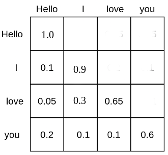
Each word token is given a probability mass at which it attends all other word tokens and, subsequently is put into relation with all other word tokens. E.g. the word “love” attends to the word “Hello” with 5%, to “I” with 30%, and to itself with 65%.

A LLM based on self-attention, but without position embeddings would have great difficulties in understanding the positions of the text inputs to one another.
It’s because the probability rating computed by ${\mathbf{Q}\mathbf{K}}^{T}mathbf\{QK\}^T$

For the LLM to grasp sentence order, a further cue is required and is often applied in the shape of positional encodings (or also called positional embeddings).
Positional encodings, encode the position of every token right into a numerical presentation that the LLM can leverage to higher understand sentence order.

The authors of the Attention Is All You Need paper introduced sinusoidal positional embeddings $\mathbf{P}={\mathbf{p}}_1,\dots ,{\mathbf{p}}_{N}mathbf\{P\}\; =\; mathbf\{p\}\_1,\; ldots,\; mathbf\{p\}\_N$

As a substitute of using fixed position embeddings, others (resembling Devlin et al.) used learned positional encodings for which the positional embeddings $\mathbf{P}mathbf\{P\}$ are learned during training.

Sinusoidal and learned position embeddings was once the predominant methods to encode sentence order into LLMs, but a few problems related to those positional encodings were found:

1. Sinusoidal and learned position embeddings are each absolute positional embeddings, i.e. encoding a novel embedding for every position id: $0,\dots ,N0,\; ldots,\; N$
2. When using learned position embeddings, the LLM must be trained on a set input length $NN$, which makes it difficult to extrapolate to an input length longer than what it was trained on.

Recently, relative positional embeddings that may tackle the above mentioned problems have change into more popular, most notably:

Each RoPE and ALiBi argue that it is best to cue the LLM about sentence order directly within the self-attention algorithm because it’s there that word tokens are put into relation with one another. More specifically, sentence order must be cued by modifying the ${\mathbf{Q}\mathbf{K}}^{T}mathbf\{QK\}^T$

Without going into too many details, RoPE notes that positional information might be encoded into query-key pairs, e.g. ${\mathbf{q}}_{i}mathbf\{q\}\_i$

$${\widehat{\mathbf{q}}}_i^T{\widehat{\mathbf{x}}}_j={\mathbf{q}}_i^T{\mathbf{R}}_{\theta ,i-j}{\mathbf{x}}_j\mathrm{.}mathbf\{hat\{q\}\}\_i^T\; mathbf\{hat\{x\}\}\_j\; =\; mathbf\{\{q\}\}\_i^T\; mathbf\{R\}\_\{theta,\; i\; -j\}\; mathbf\{\{x\}\}\_j.$$

By doing so, the propability rating between ${\mathbf{q}}_{i}mathbf\{q\}\_i$

RoPE is utilized in multiple of today’s most significant LLMs, resembling:

As a substitute, ALiBi proposes a much simpler relative position encoding scheme. The relative distance that input tokens have to one another is added as a negative integer scaled by a pre-defined value m to every query-key entry of the ${\mathbf{Q}\mathbf{K}}^{T}mathbf\{QK\}^T$

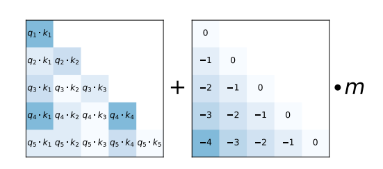
As shown within the ALiBi paper, this easy relative positional encoding allows the model to retain a high performance even at very long text input sequences.

ALiBi is utilized in multiple of today’s most significant LLMs, resembling:

Each RoPE and ALiBi position encodings can extrapolate to input lengths not seen during training whereas it has been shown that extrapolation works a lot better out-of-the-box for ALiBi as in comparison with RoPE.
For ALiBi, one simply increases the values of the lower triangular position matrix to match the length of the input sequence.
For RoPE, keeping the identical $\theta theta$ that was used during training results in poor results when passing text inputs for much longer than those seen during training, c.f Press et al.. Nonetheless, the community has found a few effective tricks that adapt $\theta theta$, thereby allowing RoPE position embeddings to work well for extrapolated text input sequences (see here).

Each RoPE and ALiBi are relative positional embeddings which can be not learned during training, but as an alternative are based on the next intuitions:

• Positional cues in regards to the text inputs must be given on to the $Q{K}^{T}QK^T$
• The LLM must be incentivized to learn a continuing relative distance positional encodings have to one another
• The further text input tokens are from one another, the lower the probability of their query-value probability. Each RoPE and ALiBi lower the query-key probability of tokens distant from one another. RoPE by decreasing their vector product by increasing the angle between the query-key vectors. ALiBi by adding large negative numbers to the vector product

In conclusion, LLMs which can be intended to be deployed in tasks that require handling large text inputs are higher trained with relative positional embeddings, resembling RoPE and ALiBi. Also note that even when an LLM with RoPE and ALiBi has been trained only on a set length of say $N_1=2048N\_1\; =\; 2048$

3.2 The important thing-value cache

Auto-regressive text generation with LLMs works by iteratively putting in an input sequence, sampling the subsequent token, appending the subsequent token to the input sequence, and continuing to achieve this until the LLM produces a token that signifies that the generation has finished.

Please have a take a look at Transformer’s Generate Text Tutorial to get a more visual explanation of how auto-regressive generation works.

Let’s run a fast code snippet to indicate how auto-regressive works in practice. We’ll simply take the most definitely next token via torch.argmax.

input_ids = tokenizer(prompt, return_tensors="pt")["input_ids"].to("cuda")

for _ in range(5):
  next_logits = model(input_ids)["logits"][:, -1:]
  next_token_id = torch.argmax(next_logits,dim=-1)

  input_ids = torch.cat([input_ids, next_token_id], dim=-1)
  print("shape of input_ids", input_ids.shape)

generated_text = tokenizer.batch_decode(input_ids[:, -5:])
generated_text

Output:

shape of input_ids torch.Size([1, 21])
shape of input_ids torch.Size([1, 22])
shape of input_ids torch.Size([1, 23])
shape of input_ids torch.Size([1, 24])
shape of input_ids torch.Size([1, 25])
[' Here is a Python function']

As we are able to see each time we increase the text input tokens by the just sampled token.

With only a few exceptions, LLMs are trained using the causal language modeling objective and subsequently mask the upper triangle matrix of the eye rating – for this reason within the two diagrams above the eye scores are left blank (a.k.a have 0 probability). For a fast recap on causal language modeling you may seek advice from the Illustrated Self Attention blog.

As a consequence, tokens never depend upon future tokens, more specifically the ${\mathbf{q}}_{i}mathbf\{q\}\_i$

In the next, we’ll tell the LLM to utilize the key-value cache by retrieving and forwarding it for every forward pass.
In Transformers, we are able to retrieve the key-value cache by passing the use_cache flag to the forward call and might then pass it with the present token.

past_key_values = None 
generated_tokens = []
next_token_id = tokenizer(prompt, return_tensors="pt")["input_ids"].to("cuda")

for _ in range(5):
  next_logits, past_key_values = model(next_token_id, past_key_values=past_key_values, use_cache=True).to_tuple()
  next_logits = next_logits[:, -1:]
  next_token_id = torch.argmax(next_logits, dim=-1)

  print("shape of input_ids", next_token_id.shape)
  
  
  
  print("variety of cached keys of the primary Transformer layer", len(past_key_values[0][0][0,0,:,:]))
  print("variety of cached values of the primary Transformer layer", len(past_key_values[0][1][0,0,:,:]))
  
  generated_tokens.append(next_token_id.item())

generated_text = tokenizer.batch_decode(generated_tokens)
generated_text

Output:

shape of input_ids torch.Size([1, 1])
variety of cached keys of the primary Transformer layer: 20
variety of cached values of the primary Transformer layer: 20
shape of input_ids torch.Size([1, 1])
variety of cached keys of the primary Transformer layer: 21
variety of cached values of the primary Transformer layer: 21
shape of input_ids torch.Size([1, 1])
variety of cached keys of the primary Transformer layer: 22
variety of cached values of the primary Transformer layer: 22
shape of input_ids torch.Size([1, 1])
variety of cached keys of the primary Transformer layer: 23
variety of cached values of the primary Transformer layer: 23
shape of input_ids torch.Size([1, 1])
variety of cached keys of the primary Transformer layer: 24
variety of cached values of the primary Transformer layer: 24
[' Here', ' is', ' a', ' Python', ' function']

As one can see, when using the key-value cache the text input tokens are not increased in length, but remain a single input vector. The length of the key-value cache alternatively is increased by one at every decoding step.

Making use of the key-value cache signifies that the ${\mathbf{Q}\mathbf{K}}^{T}mathbf\{QK\}^T$

Using the key-value cache has two benefits:

• Significant increase in computational efficiency as less computations are performed in comparison with computing the complete ${\mathbf{Q}\mathbf{K}}^{T}mathbf\{QK\}^T$
• The utmost required memory is just not increased quadratically with the variety of generated tokens, but only increases linearly.

One should at all times make use of the key-value cache because it results in similar results and a big speed-up for longer input sequences. Transformers has the key-value cache enabled by default when making use of the text pipeline or the generate method.

Note that the key-value cache is very useful for applications resembling chat where multiple passes of auto-regressive decoding are required. Let us take a look at an example.

User: How many individuals live in France?
Assistant: Roughly 75 million people live in France
User: And what number of are in Germany?
Assistant: Germany has ca. 81 million inhabitants

On this chat, the LLM runs auto-regressive decoding twice:

• 1. The primary time, the key-value cache is empty and the input prompt is "User: How many individuals live in France?" and the model auto-regressively generates the text "Roughly 75 million people live in France" while increasing the key-value cache at every decoding step.
• 2. The second time the input prompt is "User: How many individuals live in France? n Assistant: Roughly 75 million people live in France n User: And what number of in Germany?". Due to the cache, all key-value vectors for the primary two sentences are already computed. Due to this fact the input prompt only consists of "User: And what number of in Germany?". While processing the shortened input prompt, it’s computed key-value vectors are concatenated to the key-value cache of the primary decoding. The second Assistant’s answer "Germany has ca. 81 million inhabitants" is then auto-regressively generated with the key-value cache consisting of encoded key-value vectors of "User: How many individuals live in France? n Assistant: Roughly 75 million people live in France n User: And what number of are in Germany?".

Two things must be noted here:

1. Keeping all of the context is crucial for LLMs deployed in chat in order that the LLM understands all of the previous context of the conversation. E.g. for the instance above the LLM needs to grasp that the user refers back to the population when asking "And what number of are in Germany".
2. The important thing-value cache is amazingly useful for chat because it allows us to repeatedly grow the encoded chat history as an alternative of getting to re-encode the chat history again from scratch (as e.g. can be the case when using an encoder-decoder architecture).

There’s nevertheless one catch. While the required peak memory for the ${\mathbf{Q}\mathbf{K}}^{T}mathbf\{QK\}^T$

Let’s compute the variety of float values that have to be stored within the key-value cache for the LLM bigcode/octocoder that we used before.
The variety of float values amounts to 2 times the sequence length times the variety of attention heads times the eye head dimension and times the variety of layers.
Computing this for our LLM at a hypothetical input sequence length of 16000 gives:

config = model.config
2 * 16_000 * config.n_layer * config.n_head * config.n_embd // config.n_head

Output:

7864320000

Roughly 8 billion float values! Storing 8 billion float values in float16 precision requires around 15 GB of RAM which is circa half as much because the model weights themselves!
Researchers have proposed two methods that allow to significantly reduce the memory cost of storing the key-value cache:

1. Multi-Query-Attention (MQA)

Multi-Query-Attention was proposed in Noam Shazeer’s Fast Transformer Decoding: One Write-Head is All You Need paper. Because the title says, Noam came upon that as an alternative of using n_head key-value projections weights, one can use a single head-value projection weight pair that’s shared across all attention heads without that the model’s performance significantly degrades.

By utilizing a single head-value projection weight pair, the important thing value vectors ${\mathbf{k}}_i,{\mathbf{v}}_{i}mathbf\{k\}\_i,\; mathbf\{v\}\_i$

As most LLMs use between 20 and 100 attention heads, MQA significantly reduces the memory consumption of the key-value cache. For the LLM utilized in this notebook we could subsequently reduce the required memory consumption from 15 GB to lower than 400 MB at an input sequence length of 16000.

Along with memory savings, MQA also results in improved computational efficiency as explained in the next.
In auto-regressive decoding, large key-value vectors have to be reloaded, concatenated with the present key-value vector pair to be then fed into the ${\mathbf{q}}_c{\mathbf{K}}^{T}mathbf\{q\}\_cmathbf\{K\}^T$

The necessary part to grasp here is that reducing the variety of key-value attention heads to 1 only is smart if a key-value cache is used. The height memory consumption of the model for a single forward pass without key-value cache stays unchanged as every attention head still has a novel query vector in order that each attention head still has a distinct ${\mathbf{Q}\mathbf{K}}^{T}mathbf\{QK\}^T$

MQA has seen wide adoption by the community and is now utilized by lots of the preferred LLMs:

Also, the checkpoint utilized in this notebook – bigcode/octocoder – makes use of MQA.

2. Grouped-Query-Attention (GQA)

Grouped-Query-Attention, as proposed by Ainslie et al. from Google, found that using MQA can often result in quality degradation in comparison with using vanilla multi-key-value head projections. The paper argues that more model performance might be kept by less drastically reducing the variety of query head projection weights. As a substitute of using only a single key-value projection weight, n < n_head key-value projection weights must be used. By selecting n to a significantly smaller value than n_head, resembling 2,4 or 8 almost the entire memory and speed gains from MQA might be kept while sacrificing less model capability and thus arguably less performance.

Furthermore, the authors of GQA came upon that existing model checkpoints might be uptrained to have a GQA architecture with as little as 5% of the unique pre-training compute. While 5% of the unique pre-training compute can still be a large amount, GQA uptraining allows existing checkpoints to be useful for longer input sequences.

GQA was only recently proposed which is why there’s less adoption on the time of writing this notebook.
Essentially the most notable application of GQA is Llama-v2.

As a conclusion, it’s strongly advisable to utilize either GQA or MQA if the LLM is deployed with auto-regressive decoding and is required to handle large input sequences as is the case for instance for chat.

Conclusion

The research community is continuously coming up with latest, nifty ways to hurry up inference time for ever-larger LLMs. For example, one such promising research direction is speculative decoding where “easy tokens” are generated by smaller, faster language models and only “hard tokens” are generated by the LLM itself. Going into more detail is out of the scope of this notebook, but might be read upon on this nice blog post.

The rationale massive LLMs resembling GPT3/4, Llama-2-70b, Claude, PaLM can run so quickly in chat-interfaces resembling Hugging Face Chat or ChatGPT is to an enormous part due to the above-mentioned improvements in precision, algorithms, and architecture.
Going forward, accelerators resembling GPUs, TPUs, etc… will only get faster and permit for more memory, but one should nevertheless at all times ensure to make use of the most effective available algorithms and architectures to get essentially the most bang to your buck 🤗