A Beginner’s Guide to Quantum Computing with Python

Quantum Mechanics is a fundamental theory in physics that explains phenomena at a microscopic scale (like atoms and subatomic particles). This “latest” (1900) field differs from Classical Physics, which describes nature at a macroscopic scale (like bodies and machines) and doesn’t apply on the quantum level.

Quantum Computing is the exploitation of properties of Quantum Mechanics to perform computations and solve problems that a classical computer can’t and never will.

Normal computers speak the binary code language: they assign a pattern of binary digits (1s and 0s) to every character and instruction, and store and process that information in bits. Even your Python code is translated into binary digits when it runs in your laptop. For instance:

The word “Hi” → “h”: 01001000 and “i”: 01101001 → 01001000 01101001

On the opposite end, quantum computers process information with qubits (quantum bits), which may be each 0 and 1 at the identical time. That makes quantum machines dramatically faster than normal ones for specific problems (i.e. probabilistic computation).

Quantum Computers

Quantum computers use atoms and electrons, as a substitute of classical silicon-based chips. Because of this, they will leverage Quantum Mechanics to perform calculations much faster than normal machines. For example, 8-bits is enough for a classical computer to represent any number between 0 and 255, but 8-qubits is enough for a quantum computer to represent every number between 0 and 255 at the identical time. Just a few hundred qubits can be enough to represent more numbers than there are atoms within the universe.

The brain of a quantum computer is a tiny qubit chip made from metals or sapphire.

Nonetheless, probably the most iconic part is the large cooling hardware made from gold that appears like a chandelier hanging inside a steel cylinder: the dilution refrigerator. It cools the chip to a temperature colder than outer space as heat destroys quantum states (mainly the colder it’s, the more accurate it gets).

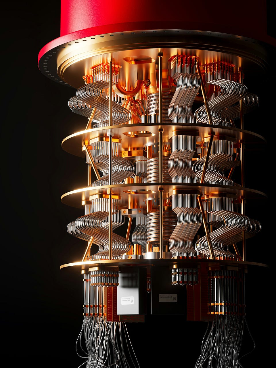
That’s the leading variety of architecture, and it’s called superconducting-qubits: artificial atoms created from circuits using superconductors (like aluminum) that exhibit zero electrical resistance at ultra-low temperatures. An alternate architecture is ion-traps (charged atoms trapped in electromagnetic fields in ultra‑high vacuum), which is more accurate but slower than the previous.

There isn’t any exact public count of what number of quantum computers are on the market, but estimates are around 200 worldwide. As of today, probably the most advanced ones are:

1. IBM’s , the most important qubit count built up to now (1000 qubits), even when that alone doesn’t equal useful computation as error rates still matter.
2. Google’s w (105 qubits), with good error rate but still removed from fault‑tolerant large‑scale computing.
3. IonQ’s (100 qubits), ion-traps quantum computer with good capabilities but still slower than superconducting machines.
4. Quantinuum’s  (98 qubits), uses ion-traps architecture with a few of the highest accuracy reported today.
5. Rigetti Computing’s (80 qubits).
6. Intel’s (12 qubits).
7. Canada Xanadu’s (12 qubits), the primary photonic quantum computer, using light as a substitute of electrons to process information.
8. Microsoft’s , the primary computer designed to scale to 1,000,000 qubits on a single chip (however it has 8 qubits in the meanwhile).
9. Chinese SpinQ’s , the primary portable small-scale quantum computer (2 qubits).
10. NVIDIA’s (), the primary GPU-accelerated quantum system.

For the time being, it’s inconceivable for a traditional person to own a large-scale quantum computer, but you possibly can access them through the cloud.

Setup

In Python, there are several libraries to work with quantum computers all over the world:

• by IBM is probably the most complete high-level ecosystem for running quantum programs on IBM quantum computers, perfect for beginners.
• by Google, dedicated to low-level control on their hardware, more suited to research.
• by Xanadu focuses on Quantum Machine Learning, it runs on their proprietary photonic computers but it may possibly hook up with other providers too.
• by ETH Zurich University, an open-source project that’s attempting to turn out to be the principal general-purpose package for quantum computing.

For this tutorial, I shall use IBM’s because it’s the industry leader (pip install qiskit).

Probably the most basic code we are able to write is to create a quantum circuit (environment for quantum computation) with just one qubit and initialize it as 0. So as to measure the state of the qubit, we’d like a statevector, which mainly tells you the present quantum reality of your circuit.

from qiskit import QuantumCircuit
from qiskit.quantum_info import Statevector

q = QuantumCircuit(1,0) #circuit with 1 quantum bit and 0 classic bit
state = Statevector.from_instruction(q) #measure state
state.probabilities() #print prob%

It means: the probability that the qubit is 0 (first element) is 100%, while the probability that the qubit is 1 (second element) is 0%. You’ll be able to print it like this:

print(f"[q=0 {round(state.probabilities()[0]*100)}%, 
         q=1 {round(state.probabilities()[1]*100)}%]")

Let’s visualize the state:

from qiskit.visualization import plot_bloch_multivector

plot_bloch_multivector(state, figsize=(3,3))

As you possibly can see from the 3D representation of the quantum state, the qubit is 100% at 0. That was the quantum equivalent of ““, and now we are able to move on to the quantum equivalent of ““.

Qubits

Qubits have two fundamental properties of Quantum Mechanics: Superposition and Entanglement.

Superposition — classical bits may be either 1 or 0, but never each. Quite the opposite, a qubit may be each (technically it’s a linear combination of an infinite variety of states between 1 and 0), and only when measured, the superposition collapses to 1 or 0 and stays like that eternally. It is because the act of observing a quantum particle forces it to tackle a classical binary state of either 1 or 0 (mainly the story of Schrödinger’s cat that everyone knows and love). Subsequently, a qubit has a certain probability of collapsing to 1 or 0.

q = QuantumCircuit(1,0)
q.h(0) #add Superposition
state = Statevector.from_instruction(q) 
print(f"[q=0 {round(state.probabilities()[0]*100)}%, 
         q=1 {round(state.probabilities()[1]*100)}%]")
plot_bloch_multivector(state, figsize=(3,3))

With the superposition, we introduced “randomness”, so the vector state is between 0 and 1. As a substitute of a vector representation, we are able to use a q-sphere where the dimensions of the points is proportional to the probability of the corresponding term within the state.

from qiskit.visualization import plot_state_qsphere

plot_state_qsphere(state, figsize=(4,4))

The qubit is each 0 and 1, with 50% of probability respectively. But what happens if we measure it? Sometimes it would be a set 1, and sometimes a set 0.

result, collapsed = state.measure() #Superposition disappears
print("measured:", result)
plot_state_qsphere(collapsed, figsize=(4,4)) #plot collapsed state

Entanglement — classical bits are independent of each other, while qubits may be entangled with one another. When that happens, qubits are eternally correlated, irrespective of the gap (often used as a mathematical metaphor for love).

q = QuantumCircuit(2,0) #circuit with 2 quantum bits and 0 classic bit
q.h([0]) #add Superposition on the first qubit
state = Statevector.from_circuit(q) 
plot_bloch_multivector(state, figsize=(3,3))

We now have the primary qubit in Superposition between 0-1, the second at 0, and now I’m going to Entangle them. Consequently, if the primary particle is measured and collapses to 1 or 0, the second particle will change as well (not necessarily to the identical result, one may be 0 while the opposite is 1).

q.cx(control_qubit=0, target_qubit=1) #Entanglement
state = Statevector.from_circuit(q)
result, collapsed = state.measure([0]) #measure the first qubit
plot_bloch_multivector(collapsed, figsize=(3,3))

As you possibly can see, the primary qubit that was on Superposition was measured and collapsed to 1. At the identical time, the second quibit is Entangled with the primary one, subsequently has modified as well.

Conclusion

This text has been a tutorial to introduce Quantum Computing basics with Python and Qiskit. We learned how one can work with qubits and their 2 fundamental properties: Superposition and Entanglement. In the following tutorial, we are going to use qubits to construct quantum models.

Full code for this text: GitHub

I hope you enjoyed it! Be happy to contact me for questions and feedback or simply to share your interesting projects.

👉 Let’s Connect 👈

_{^{(All images are by the writer unless otherwise noted)}}