

![]()
!pip install transformers==4.2.1
!pip install sentencepiece==0.1.95
The transformer-based encoder-decoder model was introduced by Vaswani
et al. within the famous Attention is all you wish
paper and is today the de-facto
standard encoder-decoder architecture in natural language processing
(NLP).
Recently, there was a variety of research on different pre-training
objectives for transformer-based encoder-decoder models, e.g. T5,
Bart, Pegasus, ProphetNet, Marge, etc…, however the model architecture
has stayed largely the identical.
The goal of the blog post is to present an in-detail explanation of
how the transformer-based encoder-decoder architecture models
sequence-to-sequence problems. We’ll give attention to the mathematical model
defined by the architecture and the way the model might be utilized in inference.
Along the way in which, we’ll give some background on sequence-to-sequence
models in NLP and break down the transformer-based encoder-decoder
architecture into its encoder and decoder parts. We offer many
illustrations and establish the link between the idea of
transformer-based encoder-decoder models and their practical usage in
🤗Transformers for inference. Note that this blog post does not explain
how such models might be trained – this can be the subject of a future blog
post.
Transformer-based encoder-decoder models are the results of years of
research on representation learning and model architectures. This
notebook provides a brief summary of the history of neural
encoder-decoder models. For more context, the reader is suggested to read
this awesome blog
post by
Sebastion Ruder. Moreover, a basic understanding of the
self-attention architecture is advisable. The next blog post by
Jay Alammar serves as refresher on the unique Transformer model
here.
On the time of writing this notebook, 🤗Transformers comprises the
encoder-decoder models T5, Bart, MarianMT, and Pegasus, which
are summarized within the docs under model
summaries.
The notebook is split into 4 parts:
- Background – A brief history of neural encoder-decoder models
is given with a give attention to RNN-based models. - Encoder-Decoder – The transformer-based encoder-decoder model
is presented and it’s explained how the model is used for
inference. - Encoder – The encoder a part of the model is explained in
detail. - Decoder – The decoder a part of the model is explained in
detail.
Each part builds upon the previous part, but may also be read on its
own.
Background
Tasks in natural language generation (NLG), a subfield of NLP, are best
expressed as sequence-to-sequence problems. Such tasks might be defined as
finding a model that maps a sequence of input words to a sequence of
goal words. Some classic examples are summarization and
translation. In the next, we assume that every word is encoded
right into a vector representation. input words can then be represented as
a sequence of input vectors:
Consequently, sequence-to-sequence problems might be solved by finding a
mapping from an input sequence of vectors to
a sequence of goal vectors , whereas the number
of goal vectors is unknown apriori and will depend on the input
sequence:
Sutskever et al. (2014) noted that
deep neural networks (DNN)s, “*despite their flexibility and power can
only define a mapping whose inputs and targets might be sensibly encoded
with vectors of fixed dimensionality.*”
Using a DNN model to unravel sequence-to-sequence problems would
subsequently mean that the variety of goal vectors must be known
apriori and would should be independent of the input . That is suboptimal because, for tasks in NLG, the
variety of goal words often will depend on the input
and not only on the input length . E.g., an article of 1000 words
might be summarized to each 200 words and 100 words depending on its
content.
In 2014, Cho et al. and
Sutskever et al. proposed to make use of an
encoder-decoder model purely based on recurrent neural networks (RNNs)
for sequence-to-sequence tasks. In contrast to DNNS, RNNs are capable
of modeling a mapping to a variable variety of goal vectors. Let’s
dive a bit deeper into the functioning of RNN-based encoder-decoder
models.
During inference, the encoder RNN encodes an input sequence by successively updating its hidden state .
After having processed the last input vector , the
encoder’s hidden state defines the input encoding . Thus,
the encoder defines the mapping:
Then, the decoder’s hidden state is initialized with the input encoding
and through inference, the decoder RNN is used to auto-regressively
generate the goal sequence. Let’s explain.
Mathematically, the decoder defines the probability distribution of a
goal sequence given the hidden state :
By Bayes’ rule the distribution might be decomposed into conditional
distributions of single goal vectors as follows:
Thus, if the architecture can model the conditional distribution of the
next goal vector, given all previous goal vectors:
then it will probably model the distribution of any goal vector sequence given
the hidden state by simply multiplying all conditional
probabilities.
So how does the RNN-based decoder architecture model ?
In computational terms, the model sequentially maps the previous inner
hidden state and the previous goal vector to the present inner hidden state and a
logit vector (shown in dark red below):
is thereby defined as being the output
hidden state of the RNN-based encoder. Subsequently, the softmax
operation is used to rework the logit vector to a
conditional probablity distribution of the following goal vector:
For more detail on the logit vector and the resulting probability
distribution, please see footnote . From the above equation, we
can see that the distribution of the present goal vector is directly conditioned on the previous goal vector and the previous hidden state .
Since the previous hidden state will depend on all
previous goal vectors , it will probably
be stated that the RNN-based decoder implicitly (e.g. not directly)
models the conditional distribution .
The space of possible goal vector sequences is
prohibitively large in order that at inference, one has to depend on decoding
methods that efficiently sample high probability goal vector
sequences from .
Given such a decoding method, during inference, the following input vector can then be sampled from
and is consequently appended to the input sequence in order that the decoder
RNN then models
to sample the following input vector and so forth in an
auto-regressive fashion.
A vital feature of RNN-based encoder-decoder models is the
definition of special vectors, reminiscent of the and vector. The vector often represents the ultimate
input vector to “cue” the encoder that the input
sequence has ended and likewise defines the top of the goal sequence. As
soon because the is sampled from a logit vector, the generation
is complete. The vector represents the input vector fed to the decoder RNN on the very first decoding step.
To output the primary logit , an input is required and since
no input has been generated at step one a special
input vector is fed to the decoder RNN. Okay – quite complicated! Let’s
illustrate and walk through an example.
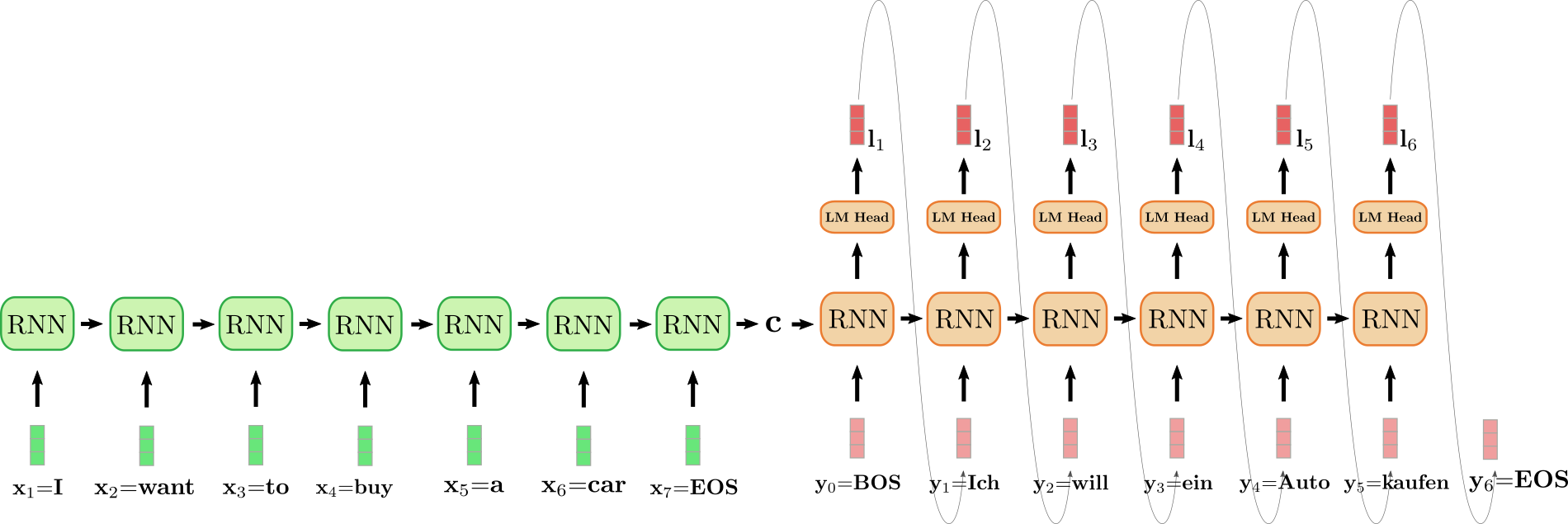
The unfolded RNN encoder is coloured in green and the unfolded RNN
decoder is coloured in red.
The English sentence “I need to purchase a automobile”, represented by , , , , , and is translated into German: “Ich will ein
Auto kaufen” defined as , , , , and . To start with, the input vector is processed by the encoder RNN and updates
its hidden state. Note that because we’re only thinking about the ultimate
encoder’s hidden state , we will disregard the RNN
encoder’s goal vector. The encoder RNN then processes the remaining of the
input sentence , , , , , in the identical fashion, updating its hidden
state at each step until the vector is reached . Within the illustration above the horizontal arrow connecting the
unfolded encoder RNN represents the sequential updates of the hidden
state. The ultimate hidden state of the encoder RNN, represented by then completely defines the encoding of the input
sequence and is used because the initial hidden state of the decoder RNN.
This might be seen as conditioning the decoder RNN on the encoded input.
To generate the primary goal vector, the decoder is fed the
vector, illustrated as within the design above. The goal
vector of the RNN is then further mapped to the logit vector via the LM Head feed-forward layer to define
the conditional distribution of the primary goal vector as explained
above:
The word is sampled (shown by the grey arrow, connecting and ) and consequently the second goal
vector might be sampled:
And so forth until at step , the vector is sampled from and the decoding is finished. The resulting goal
sequence amounts to , which is
“Ich will ein Auto kaufen” in our example above.
To sum it up, an RNN-based encoder-decoder model, represented by and defines
the distribution by
factorization:
During inference, efficient decoding methods can auto-regressively
generate the goal sequence .
The RNN-based encoder-decoder model took the NLG community by storm. In
2016, Google announced to completely replace its heavily feature engineered
translation service by a single RNN-based encoder-decoder model (see
here).
Nevertheless, RNN-based encoder-decoder models have two pitfalls. First,
RNNs suffer from the vanishing gradient problem, making it very
difficult to capture long-range dependencies, cf. Hochreiter et al.
(2001). Second,
the inherent recurrent architecture of RNNs prevents efficient
parallelization when encoding, cf. Vaswani et al.
(2017).
The unique quote from the paper is “Despite their flexibility
and power, DNNs can only be applied to problems whose inputs and targets
might be sensibly encoded with vectors of fixed dimensionality“, which
is barely adapted here.
The identical holds essentially true for convolutional neural networks
(CNNs). While an input sequence of variable length might be fed right into a
CNN, the dimensionality of the goal will at all times be depending on the
input dimensionality or fixed to a selected value.
At step one, the hidden state is initialized as a zero
vector and fed to the RNN along with the primary input vector .
A neural network can define a probability distribution over all
words, i.e. as
follows. First, the network defines a mapping from the inputs to an embedded vector representation , which corresponds to the RNN goal vector. The embedded
vector representation is then passed to the “language
model head” layer, which suggests that it’s multiplied by the word
embedding matrix, i.e. , in order that a rating
between and every encoded vector is computed. The resulting
vector is named the logit vector and might be
mapped to a probability distribution over all words by applying a
softmax operation: .
Beam-search decoding is an example of such a decoding method.
Different decoding methods are out of scope for this notebook. The
reader is suggested to seek advice from this interactive
notebook on decoding
methods.
Sutskever et al. (2014)
reverses the order of the input in order that within the above example the input
vectors would correspond to , , , , , and . The
motivation is to permit for a shorter connection between corresponding
word pairs reminiscent of and . The research group emphasizes that the
reversal of the input sequence was a key reason for his or her model’s
improved performance on machine translation.
Encoder-Decoder
In 2017, Vaswani et al. introduced the Transformer and thereby gave
birth to transformer-based encoder-decoder models.
Analogous to RNN-based encoder-decoder models, transformer-based
encoder-decoder models consist of an encoder and a decoder that are
each stacks of residual attention blocks. The important thing innovation of
transformer-based encoder-decoder models is that such residual attention
blocks can process an input sequence of variable
length without exhibiting a recurrent structure. Not counting on a
recurrent structure allows transformer-based encoder-decoders to be
highly parallelizable, which makes the model orders of magnitude more
computationally efficient than RNN-based encoder-decoder models on
modern hardware.
As a reminder, to unravel a sequence-to-sequence problem, we want to
discover a mapping of an input sequence to an output
sequence of variable length . Let’s have a look at how
transformer-based encoder-decoder models are used to seek out such a
mapping.
Much like RNN-based encoder-decoder models, the transformer-based
encoder-decoder models define a conditional distribution of goal
vectors given an input sequence :
The transformer-based encoder part encodes the input sequence to a sequence of hidden states , thus defining the mapping:
The transformer-based decoder part then models the conditional
probability distribution of the goal vector sequence given the sequence of encoded hidden states :
By Bayes’ rule, this distribution might be factorized to a product of
conditional probability distribution of the goal vector
given the encoded hidden states and all
previous goal vectors :
The transformer-based decoder hereby maps the sequence of encoded hidden
states and all previous goal vectors to the logit vector . The logit
vector is then processed by the softmax operation to
define the conditional distribution ,
just because it is finished for RNN-based decoders. Nonetheless, in contrast to
RNN-based decoders, the distribution of the goal vector
is explicitly (or directly) conditioned on all previous goal vectors as we’ll see later in additional
detail. The 0th goal vector is hereby represented by a
special “begin-of-sentence” vector.
Having defined the conditional distribution ,
we will now auto-regressively generate the output and thus define a
mapping of an input sequence to an output sequence at inference.
Let’s visualize the entire technique of auto-regressive generation of
transformer-based encoder-decoder models.
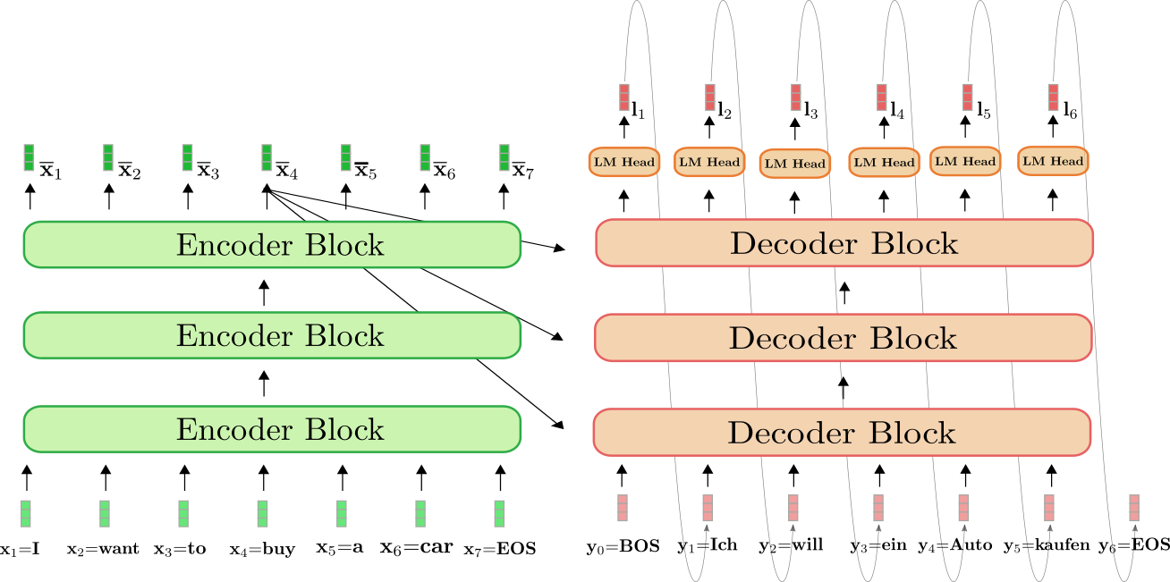
The transformer-based encoder is coloured in green and the
transformer-based decoder is coloured in red. As within the previous section,
we show how the English sentence “I need to purchase a automobile”, represented by , , , , , , and is translated into German: “Ich will ein
Auto kaufen” defined as , , , , , and .
To start with, the encoder processes the entire input sequence = “I need to purchase a automobile” (represented by the sunshine
green vectors) to a contextualized encoded sequence . E.g. defines
an encoding that depends not only on the input = “buy”,
but in addition on all other words “I”, “want”, “to”, “a”, “automobile” and
“EOS”, i.e. the context.
Next, the input encoding along with the
BOS vector, i.e. , is fed to the decoder. The decoder
processes the inputs and to
the primary logit (shown in darker red) to define the
conditional distribution of the primary goal vector :
Next, the primary goal vector = is sampled
from the distribution (represented by the grey arrows) and might now be
fed to the decoder again. The decoder now processes each
= “BOS” and = “Ich” to define the conditional
distribution of the second goal vector :
We are able to sample again and produce the goal vector =
“will”. We proceed in auto-regressive fashion until at step 6 the EOS
vector is sampled from the conditional distribution:
And so forth in auto-regressive fashion.
It is crucial to know that the encoder is simply utilized in the primary
forward pass to map to .
As of the second forward pass, the decoder can directly make use of the
previously calculated encoding . For
clarity, let’s illustrate the primary and the second forward pass for our
example above.
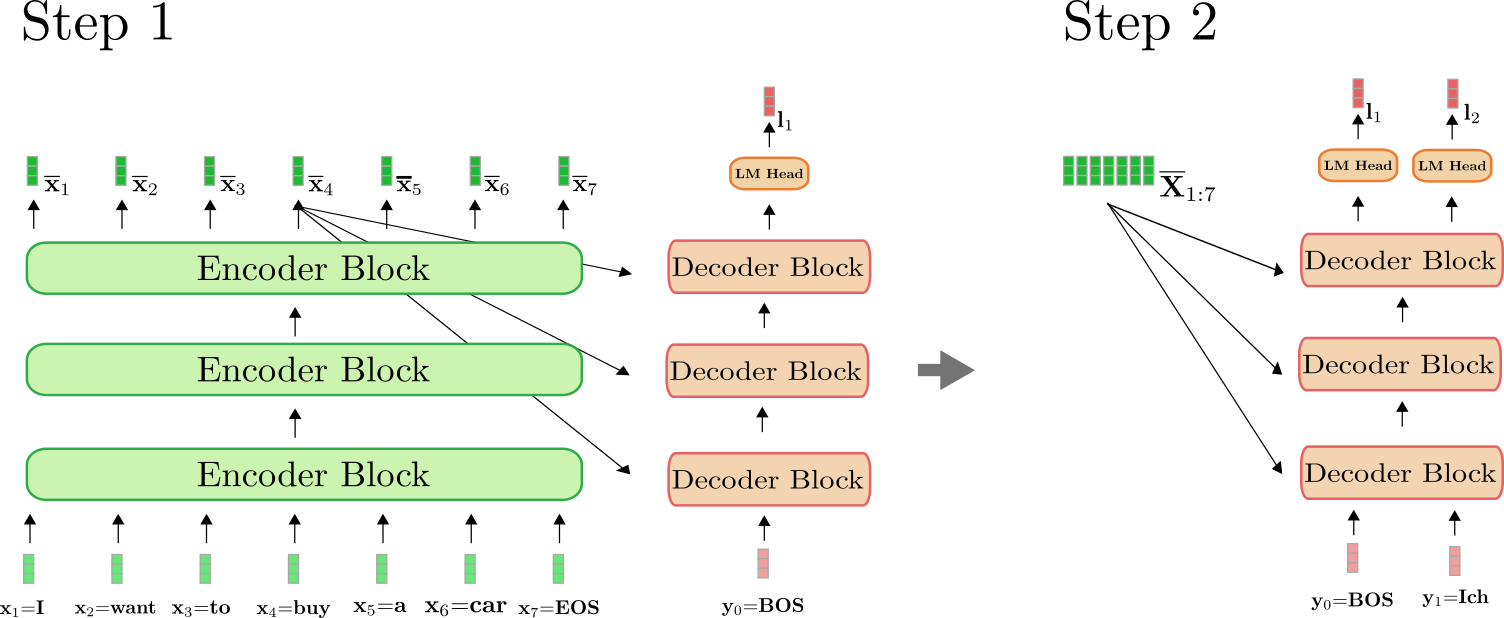
As might be seen, only in step do we have now to encode “I need to purchase
a automobile EOS” to . At step , the
contextualized encodings of “I need to purchase a automobile EOS” are simply
reused by the decoder.
In 🤗Transformers, this auto-regressive generation is finished under-the-hood
when calling the .generate() method. Let’s use considered one of our translation
models to see this in motion.
from transformers import MarianMTModel, MarianTokenizer

tokenizer = MarianTokenizer.from_pretrained("Helsinki-NLP/opus-mt-en-de")
model = MarianMTModel.from_pretrained("Helsinki-NLP/opus-mt-en-de")


input_ids = tokenizer("I need to purchase a automobile", return_tensors="pt").input_ids


output_ids = model.generate(input_ids)[0]


print(tokenizer.decode(output_ids))
Output:
Ich will ein Auto kaufen
Calling .generate() does many things under-the-hood. First, it passes
the input_ids to the encoder. Second, it passes a pre-defined token, which is the symbol within the case of
MarianMTModel together with the encoded input_ids to the decoder.
Third, it applies the beam search decoding mechanism to
auto-regressively sample the following output word of the last decoder
output . For more detail on how beam search decoding works, one is
advised to read this blog
post.
Within the Appendix, we have now included a code snippet that shows how a straightforward
generation method might be implemented “from scratch”. To totally
understand how auto-regressive generation works under-the-hood, it’s
highly advisable to read the Appendix.
To sum it up:
- The transformer-based encoder defines a mapping from the input
sequence to a contextualized encoding sequence
. - The transformer-based decoder defines the conditional distribution
. - Given an appropriate decoding mechanism, the output sequence
can auto-regressively be sampled from
.
Great, now that we have now gotten a general overview of how
transformer-based encoder-decoder models work, we will dive deeper into
each the encoder and decoder a part of the model. More specifically, we
will see exactly how the encoder makes use of the self-attention layer
to yield a sequence of context-dependent vector encodings and the way
self-attention layers allow for efficient parallelization. Then, we’ll
explain intimately how the self-attention layer works within the decoder
model and the way the decoder is conditioned on the encoder’s output with
cross-attention layers to define the conditional distribution .
Along, the way in which it would develop into obvious how transformer-based
encoder-decoder models solve the long-range dependencies problem of
RNN-based encoder-decoder models.
Within the case of "Helsinki-NLP/opus-mt-en-de", the decoding
parameters might be accessed
here,
where we will see that model applies beam search with num_beams=6.
Encoder
As mentioned within the previous section, the transformer-based encoder
maps the input sequence to a contextualized encoding sequence:
Taking a better have a look at the architecture, the transformer-based encoder
is a stack of residual encoder blocks. Each encoder block consists of
a bi-directional self-attention layer, followed by two feed-forward
layers. For simplicity, we disregard the normalization layers on this
notebook. Also, we won’t further discuss the role of the 2
feed-forward layers, but simply see it as a final vector-to-vector
mapping required in each encoder block . The bi-directional
self-attention layer puts each input vector into relation with all
input vectors and by doing so
transforms the input vector to a more “refined”
contextual representation of itself, defined as .
Thereby, the primary encoder block transforms each input vector of the
input sequence (shown in light green below) from a
context-independent vector representation to a context-dependent
vector representation, and the next encoder blocks further refine
this contextual representation until the last encoder block outputs the
final contextual encoding (shown in darker
green below).
Let’s visualize how the encoder processes the input sequence “I need
to purchase a automobile EOS” to a contextualized encoding sequence. Much like
RNN-based encoders, transformer-based encoders also add a special
“end-of-sequence” input vector to the input sequence to hint to the
model that the input vector sequence is finished .
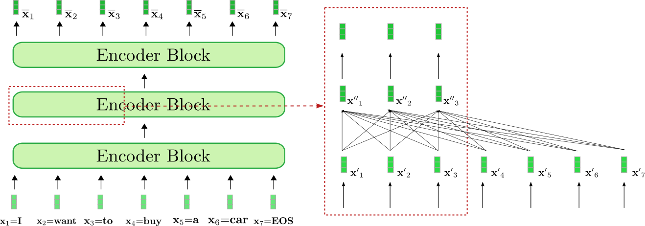
Our exemplary transformer-based encoder consists of three encoder
blocks, whereas the second encoder block is shown in additional detail within the
red box on the correct for the primary three input vectors . The bi-directional
self-attention mechanism is illustrated by the fully-connected graph in
the lower a part of the red box and the 2 feed-forward layers are shown
within the upper a part of the red box. As stated before, we’ll focus only
on the bi-directional self-attention mechanism.
As might be seen each output vector of the self-attention layer depends directly on
all input vectors . This implies,
e.g. that the input vector representation of the word “want”, i.e. , is put into direct relation with the word “buy”,
i.e. , but in addition with the word “I”,i.e. . The output vector representation of “want”, i.e. , thus represents a more refined contextual
representation for the word “want”.
Let’s take a deeper have a look at how bi-directional self-attention works.
Each input vector of an input sequence of an encoder block is projected to a key vector , value vector and query vector (shown in orange, blue, and purple respectively below)
through three trainable weight matrices :
Note, that the same weight matrices are applied to every input vector . After projecting each
input vector to a question, key, and value vector, each
query vector is compared
to all key vectors . The more
similar considered one of the important thing vectors is to
a question vector , the more essential is the corresponding
value vector for the output vector . More
specifically, an output vector is defined because the
weighted sum of all value vectors
plus the input vector . Thereby, the weights are
proportional to the cosine similarity between and the
respective key vectors , which is
mathematically expressed by as
illustrated within the equation below. For an entire description of the
self-attention layer, the reader is suggested to check out
this blog post or
the unique paper.
Alright, this sounds quite complicated. Let’s illustrate the
bi-directional self-attention layer for considered one of the query vectors of our
example above. For simplicity, it’s assumed that our exemplary
transformer-based decoder uses only a single attention head
config.num_heads = 1 and that no normalization is applied.
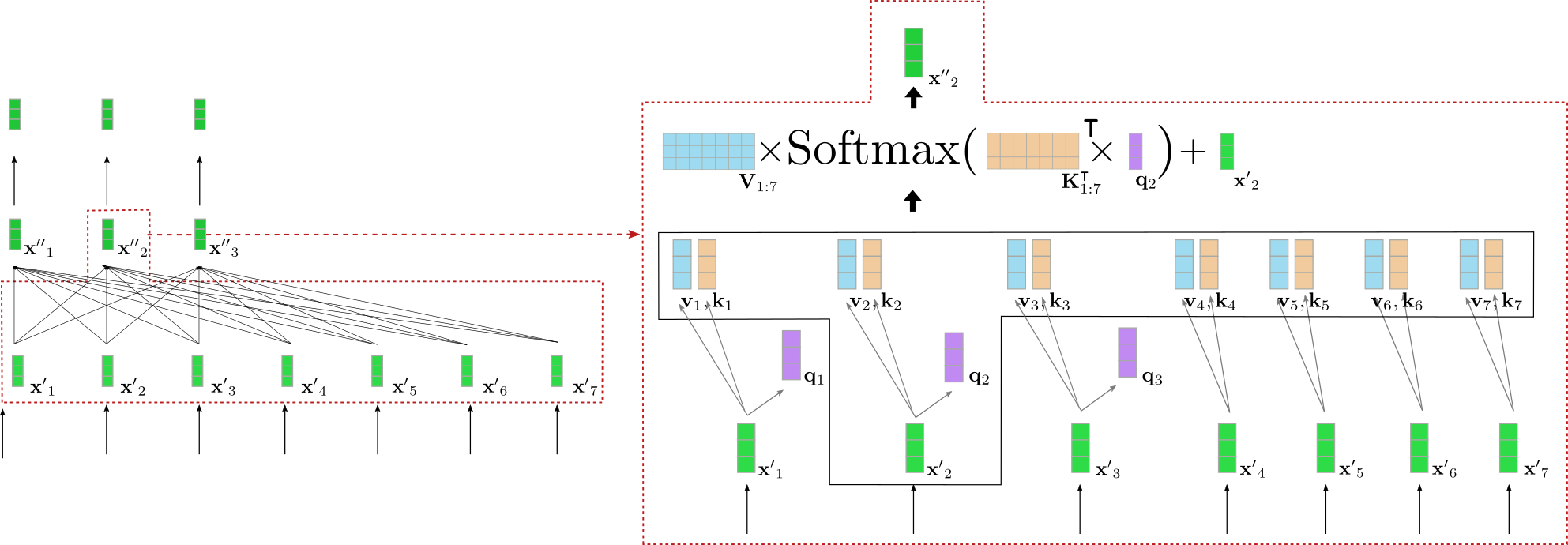
On the left, the previously illustrated second encoder block is shown
again and on the correct, an intimately visualization of the bi-directional
self-attention mechanism is given for the second input vector that corresponds to the input word “want”. At first
all input vectors are projected
to their respective query vectors
(only the primary three query vectors are shown in purple above), value
vectors (shown in blue), and key
vectors (shown in orange). The
query vector is then multiplied by the transpose of all
key vectors, i.e. followed by the
softmax operation to yield the self-attention weights. The
self-attention weights are finally multiplied by the respective value
vectors and the input vector is added to output the
“refined” representation of the word “want”, i.e.
(shown in dark green on the correct). The entire equation is illustrated in
the upper a part of the box on the correct. The multiplication of and thereby makes it
possible to match the vector representation of “want” to all other
input vector representations “I”, “to”, “buy”, “a”, “automobile”,
“EOS” in order that the self-attention weights mirror the importance each of
the opposite input vector representations for the refined representation of the word “want”.
To further understand the implications of the bi-directional
self-attention layer, let’s assume the next sentence is processed:
“The home is gorgeous and well positioned in the midst of town
where it is definitely accessible by public transport“. The word “it”
refers to “house”, which is 12 “positions away”. In
transformer-based encoders, the bi-directional self-attention layer
performs a single mathematical operation to place the input vector of
“house” into relation with the input vector of “it” (compare to the
first illustration of this section). In contrast, in an RNN-based
encoder, a word that’s 12 “positions away”, would require no less than 12
mathematical operations meaning that in an RNN-based encoder a linear
variety of mathematical operations are required. This makes it much
harder for an RNN-based encoder to model long-range contextual
representations. Also, it becomes clear that a transformer-based encoder
is far less vulnerable to lose essential information than an RNN-based
encoder-decoder model since the sequence length of the encoding is
kept the identical, i.e. ,
while an RNN compresses the length from to only , which makes it very difficult for RNNs
to effectively encode long-range dependencies between input words.
Along with making long-range dependencies more easily learnable, we
can see that the Transformer architecture is capable of process text in
parallel.Mathematically, this will easily be shown by writing the
self-attention formula as a product of query, key, and value matrices:
The output
is computed via a series of matrix multiplications and a softmax
operation, which might be parallelized effectively. Note, that in an
RNN-based encoder model, the computation of the hidden state must be done sequentially: Compute hidden state of the
first input vector , then compute the hidden state of the
second input vector that will depend on the hidden state of the primary hidden
vector, etc. The sequential nature of RNNs prevents effective
parallelization and makes them rather more inefficient in comparison with
transformer-based encoder models on modern GPU hardware.
Great, now we should always have a greater understanding of a) how
transformer-based encoder models effectively model long-range contextual
representations and b) how they efficiently process long sequences of
input vectors.
Now, let’s code up a brief example of the encoder a part of our
MarianMT encoder-decoder models to confirm that the explained theory
holds in practice.
An in-detail explanation of the role the feed-forward layers play
in transformer-based models is out-of-scope for this notebook. It’s
argued in Yun et. al, (2017)
that feed-forward layers are crucial to map each contextual vector individually to the specified output space, which the
self-attention layer doesn’t manage to do by itself. It needs to be
noted here, that every output token is processed by the
same feed-forward layer. For more detail, the reader is suggested to read
the paper.
Nonetheless, the EOS input vector doesn’t should be appended to the
input sequence, but has been shown to enhance performance in lots of cases.
In contrast to the 0th goal vector of the
transformer-based decoder is required as a starting input vector to
predict a primary goal vector.
from transformers import MarianMTModel, MarianTokenizer
import torch

tokenizer = MarianTokenizer.from_pretrained("Helsinki-NLP/opus-mt-en-de")
model = MarianMTModel.from_pretrained("Helsinki-NLP/opus-mt-en-de")

embeddings = model.get_input_embeddings()


input_ids = tokenizer("I need to purchase a automobile", return_tensors="pt").input_ids


encoder_hidden_states = model.base_model.encoder(input_ids, return_dict=True).last_hidden_state


input_ids_perturbed = tokenizer("I need to purchase a house", return_tensors="pt").input_ids
encoder_hidden_states_perturbed = model.base_model.encoder(input_ids_perturbed, return_dict=True).last_hidden_state


print(f"Length of input embeddings {embeddings(input_ids).shape[1]}. Length of encoder_hidden_states {encoder_hidden_states.shape[1]}")


print("Is encoding for `I` equal to its perturbed version?: ", torch.allclose(encoder_hidden_states[0, 0], encoder_hidden_states_perturbed[0, 0], atol=1e-3))
Outputs:
    Length of input embeddings 7. Length of encoder_hidden_states 7
    Is encoding for `I` equal to its perturbed version?:  False
We compare the length of the input word embeddings, i.e.
embeddings(input_ids) corresponding to , with the
length of the encoder_hidden_states, corresponding to . Also, we have now forwarded the word sequence
“I need to purchase a automobile” and a rather perturbated version “I need to
buy a house” through the encoder to ascertain if the primary output encoding,
corresponding to “I”, differs when only the last word is modified in
the input sequence.
As expected the output length of the input word embeddings and encoder
output encodings, i.e. and , is equal. Second, it will probably be
noted that the values of the encoded output vector of are different when the last word
is modified from “automobile” to “house”. This nonetheless shouldn’t come as a
surprise if one has understood bi-directional self-attention.
On a side-note, autoencoding models, reminiscent of BERT, have the very same
architecture as transformer-based encoder models. Autoencoding
models leverage this architecture for large self-supervised
pre-training on open-domain text data in order that they will map any word
sequence to a deep bi-directional representation. In Devlin et al.
(2018), the authors show that a
pre-trained BERT model with a single task-specific classification layer
on top can achieve SOTA results on eleven NLP tasks. All autoencoding
models of 🤗Transformers might be found
here.
Decoder
As mentioned within the Encoder-Decoder section, the transformer-based
decoder defines the conditional probability distribution of a goal
sequence given the contextualized encoding sequence:
which by Bayes’ rule might be decomposed right into a product of conditional
distributions of the following goal vector given the contextualized
encoding sequence and all previous goal vectors:
Let’s first understand how the transformer-based decoder defines a
probability distribution. The transformer-based decoder is a stack of
decoder blocks followed by a dense layer, the “LM head”. The stack
of decoder blocks maps the contextualized encoding sequence and a goal vector sequence prepended by
the vector and cut to the last goal vector, i.e. , to an encoded sequence of goal vectors . Then, the “LM head” maps the encoded
sequence of goal vectors to a
sequence of logit vectors , whereas the
dimensionality of every logit vector corresponds to the
size of the vocabulary. This manner, for every a
probability distribution over the entire vocabulary might be obtained by
applying a softmax operation on . These distributions
define the conditional distribution:
respectively. The “LM head” is commonly tied to the transpose of the word
embedding matrix, i.e. . Intuitively which means that for all
the “LM Head” layer compares the encoded output vector to all word embeddings within the vocabulary in order that the logit
vector represents the similarity scores between the
encoded output vector and every word embedding. The softmax operation
simply transformers the similarity scores to a probability distribution.
For every , the next equations hold:
Putting all of it together, with the intention to model the conditional distribution
of a goal vector sequence , the goal vectors prepended by the special vector,
i.e. , are first mapped along with the contextualized
encoding sequence to the logit vector
sequence . Consequently, each logit goal vector is transformed right into a conditional probability
distribution of the goal vector using the softmax
operation. Finally, the conditional probabilities of all goal vectors multiplied together to yield the
conditional probability of the entire goal vector sequence:
In contrast to transformer-based encoders, in transformer-based
decoders, the encoded output vector needs to be
representation of the next goal vector and
not of the input vector itself. Moreover, the encoded output vector needs to be conditioned on all contextualized
encoding sequence . To satisfy these
requirements each decoder block consists of a uni-directional
self-attention layer, followed by a cross-attention layer and two
feed-forward layers . The uni-directional self-attention layer
puts each of its input vectors only into relation with
all previous input vectors for
all to model the probability distribution of
the following goal vectors. The cross-attention layer puts each of its
input vectors into relation with all contextualized
encoding vectors to condition the
probability distribution of the following goal vectors on the input of the
encoder as well.
Alright, let’s visualize the transformer-based decoder for our
English to German translation example.
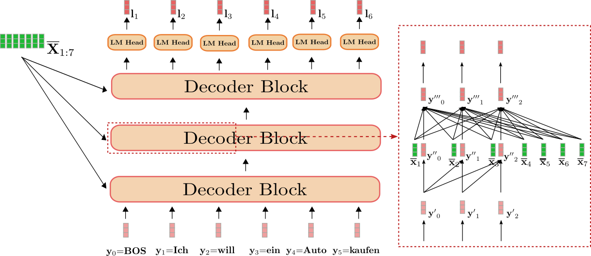
We are able to see that the decoder maps the input “BOS”,
“Ich”, “will”, “ein”, “Auto”, “kaufen” (shown in light red)
along with the contextualized sequence of “I”, “want”, “to”,
“buy”, “a”, “automobile”, “EOS”, i.e.
(shown in dark green) to the logit vectors (shown in
dark red).
Applying a softmax operation on each can thus define the
conditional probability distributions:
The general conditional probability of:
can subsequently be computed as the next product:
The red box on the correct shows a decoder block for the primary three
goal vectors . Within the lower
part, the uni-directional self-attention mechanism is illustrated and in
the center, the cross-attention mechanism is illustrated. Let’s first
give attention to uni-directional self-attention.
As in bi-directional self-attention, in uni-directional self-attention,
the query vectors (shown in
purple below), key vectors
(shown in orange below), and value vectors (shown in blue below) are
projected from their respective input vectors (shown in light red below).
Nonetheless, in uni-directional self-attention, each query vector is compared only to its respective key vector and all
previous ones, namely to yield the
respective attention weights. This prevents an output vector (shown in dark red below) to incorporate any information
in regards to the following input vector for
all . As is the case in bi-directional
self-attention, the eye weights are then multiplied by their
respective value vectors and summed together.
We are able to summarize uni-directional self-attention as follows:
Note that the index range of the important thing and value vectors is as a substitute
of which can be the range of the important thing vectors in
bi-directional self-attention.
Let’s illustrate uni-directional self-attention for the input vector for our example above.
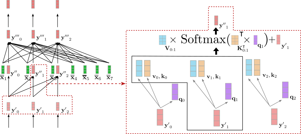
As might be seen only will depend on and . Due to this fact, we put the vector representation of the word
“Ich”, i.e. only into relation with itself and the
“BOS” goal vector, i.e. , but not with the
vector representation of the word “will”, i.e. .
So why is it essential that we use uni-directional self-attention within the
decoder as a substitute of bi-directional self-attention? As stated above, a
transformer-based decoder defines a mapping from a sequence of input
vector to the logits corresponding to the next
decoder input vectors, namely . In our example, this
means, e.g. that the input vector = “Ich” is mapped
to the logit vector , which is then used to predict the
input vector . Thus, if would have access
to the next input vectors , the decoder would
simply copy the vector representation of “will”, i.e. , to be its output . This could be
forwarded to the last layer in order that the encoded output vector would essentially just correspond to the
vector representation .
This is clearly disadvantageous because the transformer-based decoder would
never learn to predict the following word given all previous words, but just
copy the goal vector through the network to for all . In
order to define a conditional distribution of the following goal vector,
the distribution can’t be conditioned on the following goal vector itself.
It doesn’t make much sense to predict from since the
distribution is conditioned on the goal vector it’s imagined to
model. The uni-directional self-attention architecture, subsequently,
allows us to define a causal probability distribution, which is
crucial to effectively model a conditional distribution of the following
goal vector.
Great! Now we will move to the layer that connects the encoder and
decoder – the cross-attention mechanism!
The cross-attention layer takes two vector sequences as inputs: the
outputs of the uni-directional self-attention layer, i.e. and the contextualized encoding vectors . As within the self-attention layer, the query
vectors are projections of the
output vectors of the previous layer, i.e. .
Nonetheless, the important thing and value vectors and are projections of the
contextualized encoding vectors . Having
defined key, value, and query vectors, a question vector is
then in comparison with all key vectors and the corresponding rating is used
to weight the respective value vectors, just as is the case for
bi-directional self-attention to present the output vector for all . Cross-attention
might be summarized as follows:
Note that the index range of the important thing and value vectors is
corresponding to the variety of contextualized encoding vectors.
Let’s visualize the cross-attention mechanism for the input
vector for our example above.
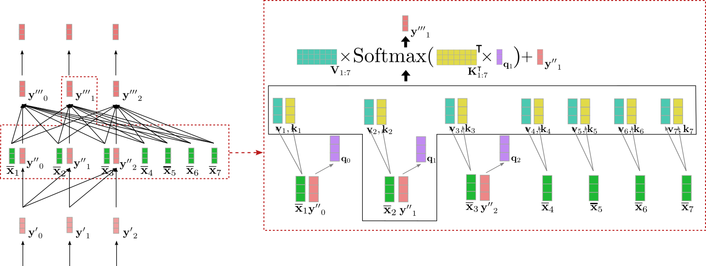
We are able to see that the query vector (shown in purple) is
derived from (shown in red) and subsequently relies on a vector
representation of the word “Ich”. The query vector
is then in comparison with the important thing vectors (shown in yellow) corresponding to
the contextual encoding representation of all encoder input vectors = “I need to purchase a automobile EOS”. This puts the vector
representation of “Ich” into direct relation with all encoder input
vectors. Finally, the eye weights are multiplied by the worth
vectors (shown in turquoise) to
yield along with the input vector the output vector (shown in dark red).
So intuitively, what happens here exactly? Each output vector is a weighted sum of all value projections of the
encoder inputs plus the input
vector itself (c.f. illustrated formula above). The important thing
mechanism to know is the next: Depending on how similar a
query projection of the input decoder vector is to a
key projection of the encoder input vector , the more
essential is the worth projection of the encoder input vector . In loose terms this implies, the more “related” a
decoder input representation is to an encoder input representation, the
more does the input representation influence the decoder output
representation.
Cool! Now we will see how this architecture nicely conditions each output
vector on the interaction between the encoder input
vectors and the input vector . One other essential remark at this point is that
the architecture is totally independent of the number of
contextualized encoding vectors on which
the output vector is conditioned on. All projection
matrices and to derive the important thing vectors and the worth vectors respectively are shared across all
positions and all value vectors are summed together to a single
weighted averaged vector. Now it becomes obvious as well, why the
transformer-based decoder doesn’t suffer from the long-range dependency
problem, the RNN-based decoder suffers from. Because each decoder logit
vector is directly depending on each encoded output vector,
the variety of mathematical operations to match the primary encoded
output vector and the last decoder logit vector amounts essentially to
only one.
To conclude, the uni-directional self-attention layer is liable for
conditioning each output vector on all previous decoder input vectors
and the present input vector and the cross-attention layer is
responsible to further condition each output vector on all encoded input
vectors.
To confirm our theoretical understanding, let’s proceed our code
example from the encoder section above.
The word embedding matrix gives each
input word a singular context-independent vector representation. This
matrix is commonly fixed because the “LM Head” layer. Nonetheless, the “LM Head”
layer can thoroughly consist of a very independent “encoded
vector-to-logit” weight mapping.
Again, an in-detail explanation of the role the feed-forward
layers play in transformer-based models is out-of-scope for this
notebook. It’s argued in Yun et. al,
(2017) that feed-forward layers
are crucial to map each contextual vector individually
to the specified output space, which the self-attention layer doesn’t
manage to do by itself. It needs to be noted here, that every output token is processed by the identical feed-forward layer. For more
detail, the reader is suggested to read the paper.
from transformers import MarianMTModel, MarianTokenizer
import torch
tokenizer = MarianTokenizer.from_pretrained("Helsinki-NLP/opus-mt-en-de")
model = MarianMTModel.from_pretrained("Helsinki-NLP/opus-mt-en-de")
embeddings = model.get_input_embeddings()
input_ids = tokenizer("I need to purchase a automobile", return_tensors="pt").input_ids
encoder_output_vectors = model.base_model.encoder(input_ids, return_dict=True).last_hidden_state
decoder_input_ids = tokenizer(" Ich will ein" , return_tensors="pt", add_special_tokens=False).input_ids
decoder_output_vectors = model.base_model.decoder(decoder_input_ids, encoder_hidden_states=encoder_output_vectors).last_hidden_state
lm_logits = torch.nn.functional.linear(decoder_output_vectors, embeddings.weight, bias=model.final_logits_bias)
decoder_input_ids_perturbed = tokenizer(" Ich will das" , return_tensors="pt", add_special_tokens=False).input_ids
decoder_output_vectors_perturbed = model.base_model.decoder(decoder_input_ids_perturbed, encoder_hidden_states=encoder_output_vectors).last_hidden_state
lm_logits_perturbed = torch.nn.functional.linear(decoder_output_vectors_perturbed, embeddings.weight, bias=model.final_logits_bias)
print(f"Shape of decoder input vectors {embeddings(decoder_input_ids).shape}. Shape of decoder logits {lm_logits.shape}")
print("Is encoding for `Ich` equal to its perturbed version?: ", torch.allclose(lm_logits[0, 0], lm_logits_perturbed[0, 0], atol=1e-3))
Output:
    Shape of decoder input vectors torch.Size([1, 5, 512]). Shape of decoder logits torch.Size([1, 5, 58101])
    Is encoding for `Ich` equal to its perturbed version?:  True
We compare the output shape of the decoder input word embeddings, i.e.
embeddings(decoder_input_ids) (corresponds to ,
here
tokens) with the dimensionality of the lm_logits(corresponds to ). Also, we have now passed the word sequence
“
“
encoder_output_vectors through the decoder to ascertain if the second
lm_logit, corresponding to “Ich”, differs when only the last word is
modified within the input sequence (“ein” -> “das”).
As expected the output shapes of the decoder input word embeddings and
lm_logits, i.e. the dimensionality of and are different within the last dimension. While the
sequence length is identical (=5), the dimensionality of a decoder input
word embedding corresponds to model.config.hidden_size, whereas the
dimensionality of a lm_logit corresponds to the vocabulary size
model.config.vocab_size, as explained above. Second, it will probably be noted
that the values of the encoded output vector of are the identical when the last word is modified
from “ein” to “das”. This nonetheless shouldn’t come as a surprise if
one has understood uni-directional self-attention.
On a final side-note, auto-regressive models, reminiscent of GPT2, have the
same architecture as transformer-based decoder models if one
removes the cross-attention layer because stand-alone auto-regressive
models will not be conditioned on any encoder outputs. So auto-regressive
models are essentially the identical as auto-encoding models but replace
bi-directional attention with uni-directional attention. These models
may also be pre-trained on massive open-domain text data to indicate
impressive performances on natural language generation (NLG) tasks. In
Radford et al.
(2019),
the authors show that a pre-trained GPT2 model can achieve SOTA or close
to SOTA results on a wide range of NLG tasks without much fine-tuning. All
auto-regressive models of 🤗Transformers might be found
here.
Alright, that is it! Now, you need to have gotten understanding of
transformer-based encoder-decoder models and find out how to use them with the
🤗Transformers library.
Thanks loads to Victor Sanh, Sasha Rush, Sam Shleifer, Oliver Åstrand,
Ted Moskovitz and Kristian Kyvik for giving useful feedback.
Appendix
As mentioned above, the next code snippet shows how one can program
a straightforward generation method for transformer-based encoder-decoder
models. Here, we implement a straightforward greedy decoding method using
torch.argmax to sample the goal vector.
from transformers import MarianMTModel, MarianTokenizer
import torch
tokenizer = MarianTokenizer.from_pretrained("Helsinki-NLP/opus-mt-en-de")
model = MarianMTModel.from_pretrained("Helsinki-NLP/opus-mt-en-de")
input_ids = tokenizer("I need to purchase a automobile", return_tensors="pt").input_ids
decoder_input_ids = tokenizer("" , add_special_tokens=False, return_tensors="pt").input_ids
assert decoder_input_ids[0, 0].item() == model.config.decoder_start_token_id, "`decoder_input_ids` should correspond to `model.config.decoder_start_token_id`"
outputs = model(input_ids, decoder_input_ids=decoder_input_ids, return_dict=True)
encoded_sequence = (outputs.encoder_last_hidden_state,)
lm_logits = outputs.logits
next_decoder_input_ids = torch.argmax(lm_logits[:, -1:], axis=-1)
decoder_input_ids = torch.cat([decoder_input_ids, next_decoder_input_ids], axis=-1)
lm_logits = model(None, encoder_outputs=encoded_sequence, decoder_input_ids=decoder_input_ids, return_dict=True).logits
next_decoder_input_ids = torch.argmax(lm_logits[:, -1:], axis=-1)
decoder_input_ids = torch.cat([decoder_input_ids, next_decoder_input_ids], axis=-1)
lm_logits = model(None, encoder_outputs=encoded_sequence, decoder_input_ids=decoder_input_ids, return_dict=True).logits
next_decoder_input_ids = torch.argmax(lm_logits[:, -1:], axis=-1)
decoder_input_ids = torch.cat([decoder_input_ids, next_decoder_input_ids], axis=-1)
print(f"Generated to this point: {tokenizer.decode(decoder_input_ids[0], skip_special_tokens=True)}")
Outputs:
Generated to this point: Ich will ein
On this code example, we show exactly what was described earlier. We
pass an input “I need to purchase a automobile” along with the
token to the encoder-decoder model and sample from the primary logit (i.e. the primary lm_logits line). Hereby, our sampling
strategy is straightforward: greedily select the following decoder input vector that
has the very best probability. In an auto-regressive fashion, we then pass
the sampled decoder input vector along with the previous inputs to
the encoder-decoder model and sample again. We repeat this a 3rd time.
Because of this, the model has generated the words “Ich will ein”. The result
is spot-on – that is the start of the right translation of the input.
In practice, more complicated decoding methods are used to sample the
lm_logits. Most of that are covered in
this blog post.