

![]()
How the Reformer uses lower than 8GB of RAM to coach on sequences of half one million tokens
The Reformer model as introduced by Kitaev, Kaiser et al. (2020) is some of the memory-efficient transformer models for long sequence modeling as of today.
Recently, long sequence modeling has experienced a surge of interest as will be seen by the numerous submissions from this 12 months alone – Beltagy et al. (2020), Roy et al. (2020), Tay et al., Wang et al. to call just a few.
The motivation behind long sequence modeling is that many tasks in NLP, e.g. summarization, query answering, require the model to process longer input sequences than models, reminiscent of BERT, are capable of handle. In tasks that require the model to process a big input sequence, long sequence models shouldn’t have to chop the input sequence to avoid memory overflow and thus have been shown to outperform standard “BERT”-like models cf. Beltagy et al. (2020).
The Reformer pushes the limit of longe sequence modeling by its ability to process as much as half one million tokens without delay as shown on this demo. As a comparison, a traditional bert-base-uncased model limits the input length to only 512 tokens. In Reformer, each a part of the usual transformer architecture is re-engineered to optimize for minimal memory requirement and not using a significant drop in performance.
The memory improvements will be attributed to 4 features which the Reformer authors introduced to the transformer world:
- Reformer Self-Attention Layer – How you can efficiently implement self-attention without being restricted to an area context?
- Chunked Feed Forward Layers – How you can get a greater time-memory trade-off for big feed forward layers?
- Reversible Residual Layers – How you can drastically reduce memory consumption in training by a sensible residual architecture?
- Axial Positional Encodings – How you can make positional encodings usable for very large input sequences?
The goal of this blog post is to present the reader an in-depth understanding of every of the 4 Reformer features mentioned above. While the reasons are focussed on the Reformer, the reader should get a greater intuition under which circumstances each of the 4 features will be effective for other transformer models as well.
The 4 sections are only loosely connected, in order that they can thoroughly be read individually.
Reformer is a component of the 🤗Transformers library. For all users of the Reformer, it is suggested to undergo this very detailed blog post to raised understand how the model works and easy methods to accurately set its configuration. All equations are accompanied by their equivalent name for the Reformer config, e.g. config., in order that the reader can quickly relate to the official docs and configuration file.
Note: Axial Positional Encodings should not explained within the official Reformer paper, but are extensively utilized in the official codebase. This blog post gives the primary in-depth explanation of Axial Positional Encodings.
1. Reformer Self-Attention Layer
Reformer uses two sorts of special self-attention layers: local self-attention layers and Locality Sensitive Hashing (LSH) self-attention layers.
To raised introduce these recent self-attention layers, we are going to briefly recap
conventional self-attention as introduced in Vaswani et al. 2017.
This blog post uses the identical notation and coloring as the favored blog post The illustrated transformer, so the reader is strongly advised to read this blog first.
Vital: While Reformer was originally introduced for causal self-attention, it may well thoroughly be used for bi-directional self-attention as well. On this post, Reformer’s self-attention is presented for bidirectional self-attention.
Recap Global Self-Attention
The core of each Transformer model is the self-attention layer. To recap the standard self-attention layer, which we discuss with here because the global self-attention layer, allow us to assume we apply a transformer layer on the embedding vector sequence where each vector is of size config.hidden_size, i.e. .
In brief, a world self-attention layer projects to the query, key and value matrices and computes the output using the softmax operation as follows:
with being of dimension (leaving out the important thing normalization factor and self-attention weights for simplicity). For more detail on the whole transformer operation, see the illustrated transformer.
Visually, we will illustrate this operation as follows for :
Note that for all visualizations batch_size and config.num_attention_heads is assumed to be 1. Some vectors, e.g. and its corresponding output vector are marked in order that LSH self-attention can later be higher explained. The presented logic can effortlessly be prolonged for multi-head self-attention (config.num_attention_{h}eads > 1). The reader is suggested to read the illustrated transformer as a reference for multi-head self-attention.
Vital to recollect is that for every output vector , the entire input sequence is processed. The tensor of the inner dot-product has an asymptotic memory complexity of which often represents the memory bottleneck in a transformer model.
This can also be the rationale why bert-base-cased has a config.max_position_embedding_size of only 512.
Local Self-Attention
Local self-attention is the plain solution to reducing the memory bottleneck, allowing us to model longer sequences with a reduced computational cost.
In local self-attention the input
is cut into chunks: each
of length config.local_chunk_length, i.e. , and subsequently global self-attention is applied on each chunk individually.
Let’s take our input sequence for again for visualization:
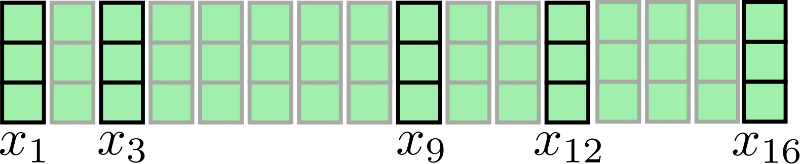
Assuming , chunked attention will be illustrated as follows:

As will be seen, the eye operation is applied for every chunk individually.
The primary drawback of this architecture becomes obvious: Some input vectors haven’t any access to their immediate context, e.g. has no access to and vice-versa in our example. That is problematic because these tokens should not capable of learn word representations that take their immediate context into consideration.
An easy treatment is to reinforce each chunk with config.local_num_chunks_before, i.e. , chunks and config.local_num_chunks_after, i.e. , in order that every input vector has no less than access to previous input vectors and following input vectors. This can be understood as chunking with overlap whereas and define the quantity of overlap each chunk has with all previous chunks and following chunks. We denote this prolonged local self-attention as follows:
with
Okay, this formula looks quite complicated. Let’s make it easier.
In Reformer’s self-attention layers is frequently set to 0 and is about to 1, so let’s write down the formula again for :
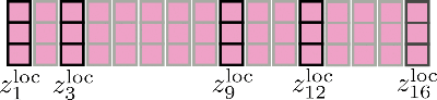
We notice that we’ve got a circular relationship in order that the primary segment can attend the last segment as well. Let’s illustrate this barely enhanced local attention again. First, we apply self-attention inside each windowed segment and keep only the central output segment.
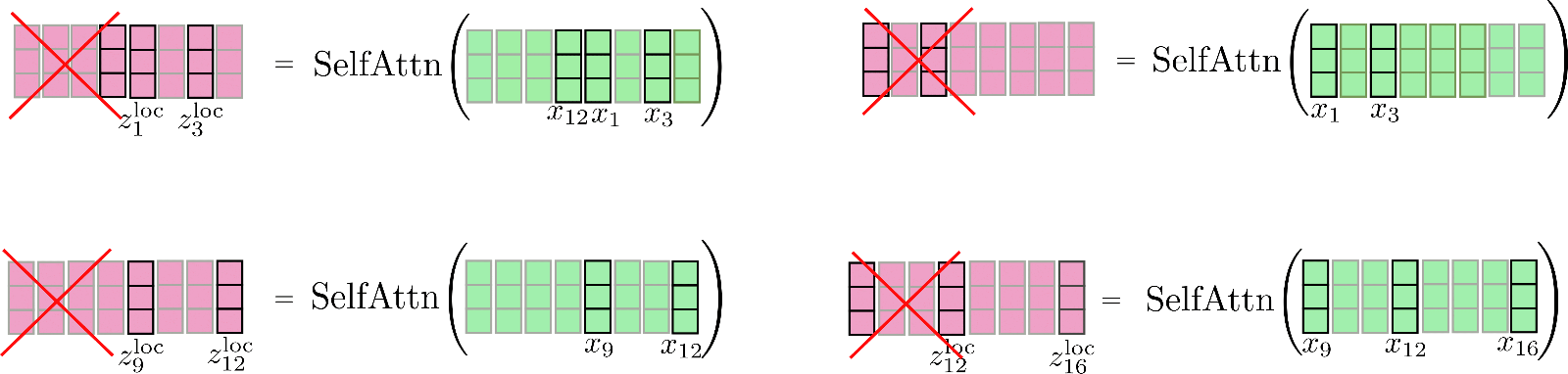
Finally, the relevant output is concatenated to and appears as follows.
Note that local self-attention is implemented efficiently way in order that no output is computed and subsequently “thrown-out” as shown here for illustration purposes by the red cross.
It is vital to notice here that extending the input vectors for every chunked self-attention function allows each single output vector of this self-attention function to learn higher vector representations. E.g. each of the output vectors can keep in mind all the input vectors to learn higher representations.
The gain in memory consumption is kind of obvious: The memory complexity is broken down for every segment individually in order that the overall asymptotic memory consumption is reduced to .
This enhanced local self-attention is best than the vanilla local self-attention architecture but still has a significant drawback in that each input vector can only attend to an area context of predefined size. For NLP tasks that don’t require the transformer model to learn long-range dependencies between the input vectors, which include arguably e.g. speech recognition, named entity recognition and causal language modeling of short sentences, this may not be an enormous issue. Many NLP tasks do require the model to learn long-range dependencies, in order that local self-attention could lead on to significant performance degradation, e.g.
- Query-answering: the model has to learn the connection between the query tokens and relevant answer tokens which can most certainly not be in the identical local range
- Multiple-Alternative: the model has to match multiple answer token segments to one another which are frequently separated by a big length
- Summarization: the model has to learn the connection between an extended sequence of context tokens and a shorter sequence of summary tokens, whereas the relevant relationships between context and summary can most certainly not be captured by local self-attention
- etc…
Local self-attention by itself is most certainly not sufficient for the transformer model to learn the relevant relationships of input vectors (tokens) to one another.
Due to this fact, Reformer moreover employs an efficient self-attention layer that approximates global self-attention, called LSH self-attention.
LSH Self-Attention
Alright, now that we’ve got understood how local self-attention works, we will take a stab on the probably most modern piece of Reformer: Locality sensitive hashing (LSH) Self-Attention.
The premise of LSH self-attention is to be roughly as efficient as local self-attention while approximating global self-attention.
LSH self-attention relies on the LSH algorithm as presented in Andoni et al (2015), hence its name.
The thought behind LSH self-attention relies on the insight that if is large, the softmax applied on the attention dot-product weights only only a few value vectors with values significantly larger than 0 for every query vector.
Let’s explain this in additional detail.
Let and be the important thing and query vectors. For every , the computation will be approximated by utilizing only those key vectors of which have a high cosine similarity with . This owes to the proven fact that the softmax function puts exponentially more weight on larger input values.
To this point so good, the following problem is to efficiently find the vectors which have a
high cosine similarity with for all .
First, the authors of Reformer notice that sharing the query and key projections: doesn’t impact the performance of a transformer model . Now, as a substitute of getting to search out the important thing vectors of high cosine similarity for every query vector , only the cosine similarity of query vectors to one another needs to be found.
This is essential because there’s a transitive property to the query-query vector dot product approximation: If has a high cosine similarity to the query vectors and , then also has a high cosine similarity to . Due to this fact, the query vectors will be clustered into buckets, such that each one query vectors that belong to the identical bucket have a high cosine similarity to one another. Let’s define because the mth set of position indices, such that their corresponding query vectors are in the identical bucket: and config.num_buckets, i.e. , because the variety of buckets.
For every set of indices , the softmax function on the corresponding bucket of query vectors approximates the softmax function of world self-attention with shared query and key projections for all position indices in .
Second, the authors make use of the LSH algorithm to cluster the query vectors right into a predefined variety of buckets . The LSH algorithm is an excellent selection here because it is extremely efficient and is an approximation of the closest neighbor algorithm for cosine similarity. Explaining the LSH scheme is out-of-scope for this notebook, so let’s just remember that for every vector the LSH algorithm attributes its position index to one among predefined buckets, i.e. with and .
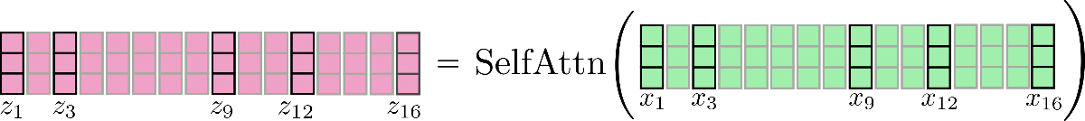
Visually, we will illustrate this as follows for our original example:

Third, it may well be noted that having clustered all query vectors in buckets, the corresponding set of indices will be used to permute the input vectors accordingly in order that shared query-key self-attention will be applied piecewise just like local attention.
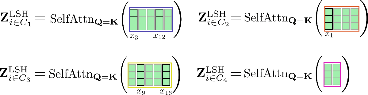
Let’s make clear with our example input vectors and assume config.num_buckets=4 and config.lsh_chunk_length = 4. Taking a look at the graphic above we will see that we’ve got assigned each query vector to one among the clusters .
If we now sort the corresponding input vectors accordingly, we get the next permuted input :

The self-attention mechanism ought to be applied for every cluster individually in order that for every cluster the corresponding output is calculated as follows: .
Let’s illustrate this again for our example.
As will be seen, the self-attention function operates on different sizes of matrices, which is suboptimal for efficient batching in GPU and TPU.
To beat this problem, the permuted input will be chunked the identical way it is completed for local attention in order that each chunk is of size config.lsh_chunk_length. By chunking the permuted input, a bucket is perhaps split into two different chunks. To treatment this problem, in LSH self-attention each chunk attends to its previous chunk config.lsh_num_chunks_before=1 along with itself, the identical way local self-attention does (config.lsh_num_chunks_after is frequently set to 0). This manner, we will be assured that each one vectors in a bucket attend to one another with a high probability .
All in all for all chunks , LSH self-attention will be noted down as follows:
with and being the input and output vectors permuted in accordance with the LSH algorithm.
Enough complicated formulas, let’s illustrate LSH self-attention.
The permuted vectors as shown above are chunked and shared query key self-attention is applied to every chunk.
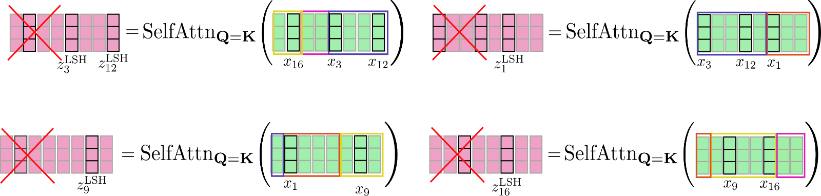
Finally, the output is reordered to its original permutation.

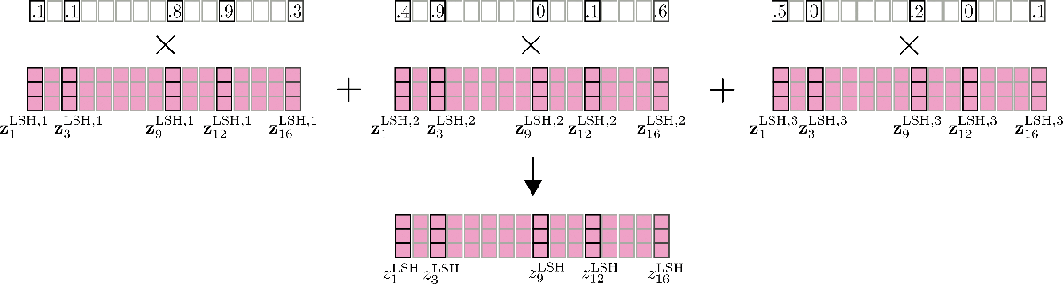
One vital feature to say here as well is that the accuracy of LSH self-attention will be improved by running LSH self-attention config.num_hashes, e.g. times in parallel, each with a special random LSH hash.
By setting config.num_hashes > 1, for every output position , multiple output vectors are computed
and subsequently merged: . The represents the importance of the output vectors of hashing round compared to the opposite hashing rounds, and is exponentially proportional to the normalization term of their softmax computation. The intuition behind that is that if the corresponding query vector have a high cosine similarity with all other query vectors in its respective chunk, then the softmax normalization term of this chunk tends to be high, in order that the corresponding output vectors ought to be a greater approximation to global attention and thus receive more weight than output vectors of hashing rounds with a lower softmax normalization term. For more detail see Appendix A of the paper. For our example, multi-round LSH self-attention will be illustrated as follows.
Great. That is it. Now we understand how LSH self-attention works in Reformer.
Regarding the memory complexity, we now have two terms that compete which one another to be the memory bottleneck: the dot-product: and the required memory for LSH bucketing: with being the chunk length. Because for big , the variety of buckets grows much faster than the chunk length , the user can again factorize the variety of buckets config.num_buckets as explained here.
Let’s recap quickly what we’ve got passed through above:
- We would like to approximate global attention using the knowledge that the softmax operation only puts significant weights on only a few key vectors.
- If key vectors are equal to question vectors which means for every query vector , the softmax only puts significant weight on other query vectors which might be similar by way of cosine similarity.
- This relationship works in each ways, meaning if is comparable to than can also be just like , in order that we will do a world clustering before applying self-attention on a permuted input.
- We apply local self-attention on the permuted input and re-order the output to its original permutation.
The authors run some preliminary experiments confirming that shared query key self-attention performs roughly in addition to standard self-attention.
To be more exact the query vectors inside a bucket are sorted in accordance with their original order. This implies if, e.g. the vectors are all hashed to bucket 2, the order of the vectors in bucket 2 would still be , followed by and .
On a side note, it’s to say the authors put a mask on the query vector to forestall the vector from attending to itself. Since the cosine similarity of a vector to itself will all the time be as high or higher than the cosine similarity to other vectors, the query vectors in shared query key self-attention are strongly discouraged to take care of themselves.
Benchmark
Benchmark tools were recently added to Transformers – see here for a more detailed explanation.
To point out how much memory will be saved using “local” + “LSH” self-attention, the Reformer model google/reformer-enwik8 is benchmarked for various local_attn_chunk_length and lsh_attn_chunk_length. The default configuration and usage of the google/reformer-enwik8 model will be checked in additional detail here.
Let’s first do some mandatory imports and installs.
#@title Installs and Imports
# pip installs
!pip -qq install git+https://github.com/huggingface/transformers.git
!pip install -qq py3nvml

from transformers import ReformerConfig, PyTorchBenchmark, PyTorchBenchmarkArguments
First, let’s benchmark the memory usage of the Reformer model using global self-attention. This will be achieved by setting lsh_attn_chunk_length = local_attn_chunk_length = 8192 in order that for all input sequences smaller or equal to 8192, the model mechanically switches to global self-attention.
config = ReformerConfig.from_pretrained("google/reformer-enwik8", lsh_attn_chunk_length=16386, local_attn_chunk_length=16386, lsh_num_chunks_before=0, local_num_chunks_before=0)
benchmark_args = PyTorchBenchmarkArguments(sequence_lengths=[2048, 4096, 8192, 16386], batch_sizes=[1], models=["Reformer"], no_speed=True, no_env_print=True)
benchmark = PyTorchBenchmark(configs=[config], args=benchmark_args)
result = benchmark.run()
HBox(children=(FloatProgress(value=0.0, description='Downloading', max=1279.0, style=ProgressStyle(description…


1 / 1
Doesn't fit on GPU. CUDA out of memory. Tried to allocate 2.00 GiB (GPU 0; 11.17 GiB total capability; 8.87 GiB already allocated; 1.92 GiB free; 8.88 GiB reserved in total by PyTorch)

====================      INFERENCE - MEMORY - RESULT       ====================
--------------------------------------------------------------------------------
          Model Name             Batch Size     Seq Length    Memory in MB
--------------------------------------------------------------------------------
           Reformer                  1              2048            1465
           Reformer                  1              4096            2757
           Reformer                  1              8192            7893
           Reformer                  1             16386            N/A
--------------------------------------------------------------------------------
The longer the input sequence, the more visible is the quadratic relationship between input sequence and peak memory usage. As will be seen, in practice it might require a for much longer input sequence to obviously observe that doubling the input sequence quadruples the height memory usage.
For this a google/reformer-enwik8 model using global attention, a sequence length of over 16K ends in a memory overflow.
Now, let’s activate local and LSH self-attention by utilizing the model’s default parameters.
  config = ReformerConfig.from_pretrained("google/reformer-enwik8")
  benchmark_args = PyTorchBenchmarkArguments(sequence_lengths=[2048, 4096, 8192, 16384, 32768, 65436], batch_sizes=[1], models=["Reformer"], no_speed=True, no_env_print=True)
  benchmark = PyTorchBenchmark(configs=[config], args=benchmark_args)
  result = benchmark.run()
1 / 1
Doesn't fit on GPU. CUDA out of memory. Tried to allocate 2.00 GiB (GPU 0; 11.17 GiB total capability; 7.85 GiB already allocated; 1.74 GiB free; 9.06 GiB reserved in total by PyTorch)
Doesn't fit on GPU. CUDA out of memory. Tried to allocate 4.00 GiB (GPU 0; 11.17 GiB total capability; 6.56 GiB already allocated; 3.99 GiB free; 6.81 GiB reserved in total by PyTorch)

====================      INFERENCE - MEMORY - RESULT       ====================
--------------------------------------------------------------------------------
          Model Name             Batch Size     Seq Length    Memory in MB
--------------------------------------------------------------------------------
           Reformer                  1              2048            1785
           Reformer                  1              4096            2621
           Reformer                  1              8192            4281
           Reformer                  1             16384            7607
           Reformer                  1             32768            N/A
           Reformer                  1             65436            N/A
--------------------------------------------------------------------------------
As expected using local and LSH self-attention is way more memory efficient for longer input sequences, in order that the model runs out of memory only at 16K tokens for a 11GB RAM GPU on this notebook.
2. Chunked Feed Forward Layers
Transformer-based models often employ very large feed forward layers after the self-attention layer in parallel. Thereby, this layer can take up a big amount of the general memory and sometimes even represent the memory bottleneck of a model.
First introduced within the Reformer paper, feed forward chunking is a way that permits to effectively trade higher memory consumption for increased time consumption.
Chunked Feed Forward Layer in Reformer
In Reformer, the LSH– or local self-attention layer is frequently followed by a residual connection, which then defines the primary part in a transformer block. For more detail on this please discuss with this blog.
The output of the primary a part of the transformer block, called normed self-attention output will be written as , with being either or in Reformer.
For our example input , we illustrate the normed self-attention output as follows.
Now, the second a part of a transformer block often consists of two feed forward layers , defined as that processes , to an intermediate output and that processes the intermediate output to the output . The 2 feed forward layers will be defined by
It will be significant to recollect at this point that mathematically the output of a feed forward layer at position only depends upon the input at this position . In contrast to the self-attention layer, every output is due to this fact completely independent of all inputs of various positions.
Let’s illustrate the feed forward layers for .
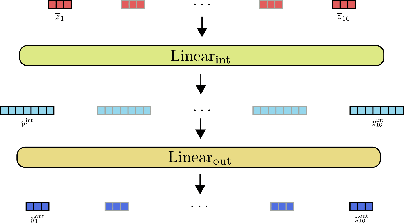
As will be depicted from the illustration, all input vectors are processed by the identical feed forward layer in parallel.
It becomes interesting when one takes a take a look at the output dimensions of the feed forward layers. In Reformer, the output dimension of is defined as config.feed_forward_size, e.g. , and the output dimension of is defined as config.hidden_size, i.e. .
The Reformer authors observed that in a transformer model the intermediate dimension often tends to be much larger than the output dimension . Which means the tensor of dimension allocates a big amount of the overall memory and may even turn out to be the memory bottleneck.
To get a greater feeling for the differences in dimensions let’s picture the matrices and for our example.
It’s becoming quite obvious that the tensor holds way more memory ( as much to be exact) than . But, is it even mandatory to compute the total intermediate matrix ? Not likely, because relevant is simply the output matrix .
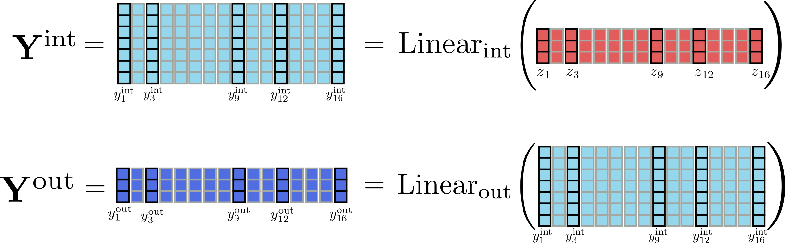
To trade memory for speed, one can thus chunk the linear layers computation to only process one chunk on the time. Defining config.chunk_size_feed_forward as , chunked linear layers are defined as with .
In practice, it just implies that the output is incrementally computed and concatenated to avoid having to store the entire intermediate tensor in memory.
Assuming for our example we will illustrate the incremental computation of the output for position as follows.
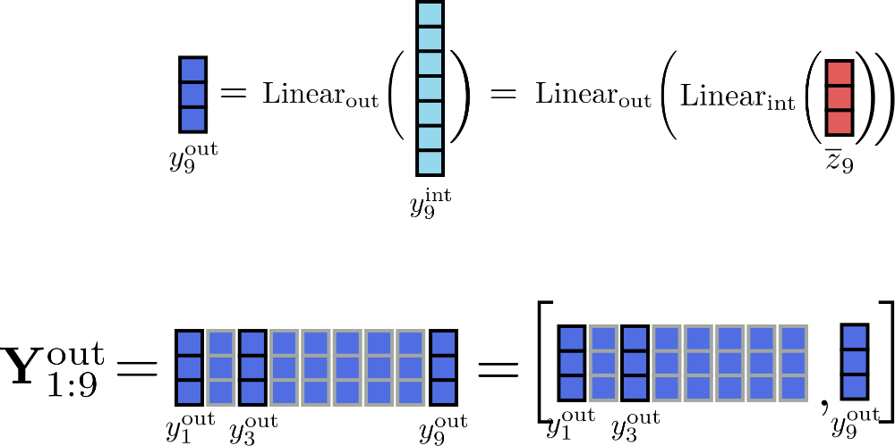
By processing the inputs in chunks of size 1, the one tensors that should be stored in memory at the identical time are of a maximum size of , of size and the input of size , with being config.hidden_size .
Finally, it can be crucial to do not forget that chunked linear layers yield a mathematically equivalent output to standard linear layers and may due to this fact be applied to all transformer linear layers. Making use of config.chunk_size_feed_forward due to this fact allows a greater trade-off between memory and speed in certain use cases.
For a less complicated explanation, the layer norm layer which is often applied to before being processed by the feed forward layers is omitted for now.
In bert-base-uncased, e.g. the intermediate dimension is with 3072 4 times larger than the output dimension .
As a reminder, the output config.num_attention_heads is assumed to be 1 for the sake of clarity and illustration on this notebook, in order that the output of the self-attention layers will be assumed to be of size config.hidden_size.
More information on chunked linear / feed forward layers can be found here on the 🤗Transformers docs.
Benchmark
Let’s test how much memory will be saved by utilizing chunked feed forward layers.
#@title Installs and Imports
# pip installs
!pip -qq install git+https://github.com/huggingface/transformers.git
!pip install -qq py3nvml

from transformers import ReformerConfig, PyTorchBenchmark, PyTorchBenchmarkArguments
Constructing wheel for transformers (setup.py) ... [?25l[?25hdone
First, let’s compare the default google/reformer-enwik8 model without chunked feed forward layers to the one with chunked feed forward layers.
config_no_chunk = ReformerConfig.from_pretrained("google/reformer-enwik8")  # no chunk
config_chunk = ReformerConfig.from_pretrained("google/reformer-enwik8", chunk_size_feed_forward=1)  # feed forward chunk
benchmark_args = PyTorchBenchmarkArguments(sequence_lengths=[1024, 2048, 4096], batch_sizes=[8], models=["Reformer-No-Chunk", "Reformer-Chunk"], no_speed=True, no_env_print=True)
benchmark = PyTorchBenchmark(configs=[config_no_chunk, config_chunk], args=benchmark_args)
result = benchmark.run()
1 / 2
Doesn't fit on GPU. CUDA out of memory. Tried to allocate 2.00 GiB (GPU 0; 11.17 GiB total capability; 7.85 GiB already allocated; 1.74 GiB free; 9.06 GiB reserved in total by PyTorch)
2 / 2
Doesn't fit on GPU. CUDA out of memory. Tried to allocate 2.00 GiB (GPU 0; 11.17 GiB total capability; 7.85 GiB already allocated; 1.24 GiB free; 9.56 GiB reserved in total by PyTorch)

====================      INFERENCE - MEMORY - RESULT       ====================
--------------------------------------------------------------------------------
          Model Name             Batch Size     Seq Length    Memory in MB
--------------------------------------------------------------------------------
      Reformer-No-Chunk              8              1024            4281
      Reformer-No-Chunk              8              2048            7607
      Reformer-No-Chunk              8              4096            N/A
        Reformer-Chunk               8              1024            4309
        Reformer-Chunk               8              2048            7669
        Reformer-Chunk               8              4096            N/A
--------------------------------------------------------------------------------
Interesting, chunked feed forward layers don’t seem to assist here in any respect. The explanation is that config.feed_forward_size isn’t sufficiently large to make an actual difference. Only at longer sequence lengths of 4096, a slight decrease in memory usage will be seen.
Let’s examine what happens to the memory peak usage if we increase the dimensions of the feed forward layer by an element of 4 and reduce the variety of attention heads also by an element of 4 in order that the feed forward layer becomes the memory bottleneck.
config_no_chunk = ReformerConfig.from_pretrained("google/reformer-enwik8", chunk_size_feed_forward=0, num_attention_{h}eads=2, feed_forward_size=16384)  # no chuck
config_chunk = ReformerConfig.from_pretrained("google/reformer-enwik8", chunk_size_feed_forward=1, num_attention_{h}eads=2, feed_forward_size=16384)  # feed forward chunk
benchmark_args = PyTorchBenchmarkArguments(sequence_lengths=[1024, 2048, 4096], batch_sizes=[8], models=["Reformer-No-Chunk", "Reformer-Chunk"], no_speed=True, no_env_print=True)
benchmark = PyTorchBenchmark(configs=[config_no_chunk, config_chunk], args=benchmark_args)
result = benchmark.run()
1 / 2
2 / 2

====================      INFERENCE - MEMORY - RESULT       ====================
--------------------------------------------------------------------------------
          Model Name             Batch Size     Seq Length    Memory in MB
--------------------------------------------------------------------------------
      Reformer-No-Chunk              8              1024            3743
      Reformer-No-Chunk              8              2048            5539
      Reformer-No-Chunk              8              4096            9087
        Reformer-Chunk               8              1024            2973
        Reformer-Chunk               8              2048            3999
        Reformer-Chunk               8              4096            6011
--------------------------------------------------------------------------------
Now a transparent decrease in peak memory usage will be seen for longer input sequences.
As a conclusion, it ought to be noted chunked feed forward layers only is sensible for models having few attention heads and huge feed forward layers.
3. Reversible Residual Layers
Reversible residual layers were first introduced in N. Gomez et al and used to scale back memory consumption when training the favored ResNet model. Mathematically, reversible residual layers are barely different
to “real” residual layers but don’t require the activations to be saved in the course of the forward pass, which may drastically reduce memory consumption for training.
Reversible Residual Layers in Reformer
Let’s start by investigating why training a model requires
way more memory than the inference of the model.
When running a model in inference, the required memory equals roughly the memory it takes to compute the single largest tensor within the model.
Then again, when training a model, the required memory equals roughly the sum of all differentiable tensors.
This isn’t surprising when considering how auto differentiation works in deep learning frameworks. These lecture slides by Roger Grosse of the University of Toronto are great to raised understand auto differentiation.
In a nutshell, to be able to calculate the gradient of a differentiable function (e.g. a layer), auto differentiation requires the gradient of the function’s output and the function’s input and output tensor. While the gradients are dynamically computed and subsequently discarded, the input and output tensors (a.k.a activations) of a function are stored in the course of the forward pass.
Alright, let’s apply this to a transformer model. A transformer model features a stack of multiple so-called transformer layers. Each additional transformer layer forces the model to store more activations in the course of the forward pass and thus increases the required memory for training.
Let’s take a more detailed look. A transformer layer essentially consists of two residual layers. The primary residual layer represents the self-attention mechanism as explained in section 1) and the second residual layer represents the linear or feed-forward layers as explained in section 2).
Using the identical notation as before, the input of a transformer layer i.e. is first normalized and subsequently processed by the self-attention layer to get the output . We’ll abbreviate these two layers with in order that .
Next, the residual is added to the input and the sum is fed into the second residual layer – the 2 linear layers. is processed by a second normalization layer, followed by the 2 linear layers to get . We’ll abbreviate the second normalization layer and the 2 linear layers with yielding .
Finally, the residual is added to to present the output of the transformer layer .
Let’s illustrate an entire transformer layer using the instance of .
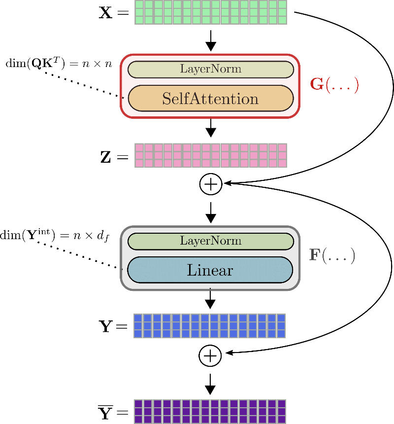
To calculate the gradient of e.g. the self-attention block , three tensors should be known beforehand: the gradient , the output , and the input . While will be calculated on-the-fly and discarded afterward, the values for and should be calculated and stored in the course of the forward pass because it isn’t possible to recalculate them easily on-the-fly during backpropagation. Due to this fact, in the course of the forward pass, large tensor outputs, reminiscent of the query-key dot product matrix or the intermediate output of the linear layers , should be stored in memory .
Here, reversible residual layers come to our help. The thought is comparatively straight-forward. The residual block is designed in a way in order that as a substitute of getting to store the input and output tensor of a function, each can easily be recalculated in the course of the backward pass in order that no tensor needs to be stored in memory in the course of the forward pass.
That is achieved by utilizing two input streams , and two output streams . The primary residual is computed by the primary output stream and subsequently added to the input of the second input stream, in order that .
Similarly, the residual is added to the primary input stream again, in order that the 2 output streams are defined by and .
The reversible transformer layer will be visualized for as follows.
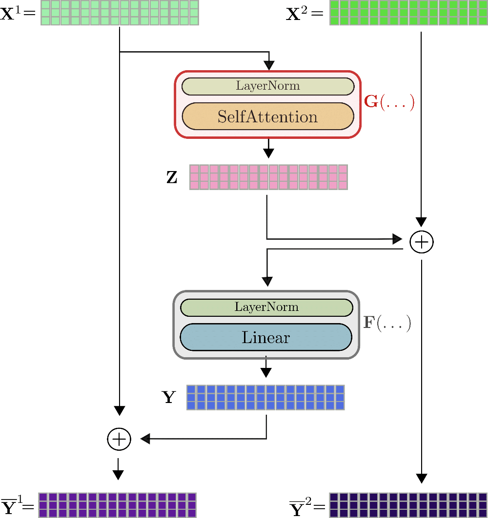
As will be seen, the outputs are calculated in a really similar way than of the non-reversible layer, but they’re mathematically different. The authors of Reformer observe in some initial experiments that the performance of a reversible transformer model matches the performance of an ordinary transformer model.
The primary visible difference to the usual transformer layer is that there are two input streams and output streams , which at first barely increases the required memory for each the forward pass.
The 2-stream architecture is crucial though for not having to save lots of any activations in the course of the forward pass. Let’s explain. For backpropagation, the reversible transformer layer has to calculate the gradients and . Along with the gradients and which will be calculated on-the-fly, the tensor values , should be known for and the tensor values and for to make auto-differentiation work.
If we assume to know , it may well easily be depicted from the graph that one can calculate as follows. . Great, now that is thought, will be computed by . Alright now, and are trivial to compute via and . In order a conclusion, if only the outputs of the last reversible transformer layer are stored in the course of the forward pass, all other relevant activations will be derived by making use of and in the course of the backward pass and passing and . The overhead of two forward passes of and per reversible transformer layer in the course of the backpropagation is traded against not having to store any activations in the course of the forward pass. Not a foul deal!
Note: Since recently, major deep learning frameworks have released code that permits to store only certain activations and recompute larger ones in the course of the backward propagation (Tensoflow here and PyTorch here). For traditional reversible layers, this still implies that no less than one activation needs to be stored for every transformer layer, but by defining which activations can dynamically be recomputed a variety of memory will be saved.
Within the previous two sections, we’ve got omitted the layer norm layers preceding each the self-attention layer and the linear layers. The reader should know that each and are each processed by layer normalization before being fed into self-attention and the linear layers respectively.
While within the design the dimension of is written as , in a LSH self-attention or local self-attention layer the dimension would only be or respectively with being the chunk length and the variety of hashes
In the primary reversible transformer layer is about to be equal to .
Benchmark
With a purpose to measure the effect of reversible residual layers, we are going to compare the memory consumption of BERT with Reformer in training for an increasing variety of layers.
#@title Installs and Imports
# pip installs
!pip -qq install git+https://github.com/huggingface/transformers.git
!pip install -qq py3nvml

from transformers import ReformerConfig, BertConfig, PyTorchBenchmark, PyTorchBenchmarkArguments
Let’s measure the required memory for the usual bert-base-uncased BERT model by increasing the variety of layers from 4 to 12.
config_4_layers_bert = BertConfig.from_pretrained("bert-base-uncased", num_hidden_layers=4)
config_8_layers_bert = BertConfig.from_pretrained("bert-base-uncased", num_hidden_layers=8)
config_12_layers_bert = BertConfig.from_pretrained("bert-base-uncased", num_hidden_layers=12)
benchmark_args = PyTorchBenchmarkArguments(sequence_lengths=[512], batch_sizes=[8], models=["Bert-4-Layers", "Bert-8-Layers", "Bert-12-Layers"], training=True, no_inference=True, no_speed=True, no_env_print=True)
benchmark = PyTorchBenchmark(configs=[config_4_layers_bert, config_8_layers_bert, config_12_layers_bert], args=benchmark_args)
result = benchmark.run()
HBox(children=(FloatProgress(value=0.0, description='Downloading', max=433.0, style=ProgressStyle(description_…


1 / 3
2 / 3
3 / 3

====================        TRAIN - MEMORY - RESULTS        ====================
--------------------------------------------------------------------------------
          Model Name             Batch Size     Seq Length    Memory in MB
--------------------------------------------------------------------------------
        Bert-4-Layers                8              512             4103
        Bert-8-Layers                8              512             5759
        Bert-12-Layers               8              512             7415
--------------------------------------------------------------------------------
It may be seen that adding a single layer of BERT linearly increases the required memory by greater than 400MB.
config_4_layers_reformer = ReformerConfig.from_pretrained("google/reformer-enwik8", num_hidden_layers=4, num_hashes=1)
config_8_layers_reformer = ReformerConfig.from_pretrained("google/reformer-enwik8", num_hidden_layers=8, num_hashes=1)
config_12_layers_reformer = ReformerConfig.from_pretrained("google/reformer-enwik8", num_hidden_layers=12, num_hashes=1)
benchmark_args = PyTorchBenchmarkArguments(sequence_lengths=[512], batch_sizes=[8], models=["Reformer-4-Layers", "Reformer-8-Layers", "Reformer-12-Layers"], training=True, no_inference=True, no_speed=True, no_env_print=True)
benchmark = PyTorchBenchmark(configs=[config_4_layers_reformer, config_8_layers_reformer, config_12_layers_reformer], args=benchmark_args)
result = benchmark.run()
1 / 3
2 / 3
3 / 3

====================        TRAIN - MEMORY - RESULTS        ====================
--------------------------------------------------------------------------------
          Model Name             Batch Size     Seq Length    Memory in MB
--------------------------------------------------------------------------------
      Reformer-4-Layers              8              512             4607
      Reformer-8-Layers              8              512             4987
      Reformer-12-Layers             8              512             5367
--------------------------------------------------------------------------------
For Reformer, alternatively, adding a layer adds significantly less memory in practice. Adding a single layer increases the required memory on average by lower than 100MB in order that a much larger 12-Layer reformer-enwik8 model requires less memory than a 12-Layer bert-base-uncased model.
4. Axial Positional Encodings
Reformer makes it possible to process huge input sequences. Nevertheless, for such long input sequences standard positional encoding weight matrices alone would use greater than 1GB to store its weights.
To stop such large positional encoding matrices, the official Reformer code introduced Axial Position Encodings.
Vital: Axial Position Encodings weren’t explained within the official paper, but will be well understood from looking into the code and talking to the authors
Axial Positional Encodings in Reformer
Transformers need positional encodings to account for the order of words within the input because self-attention layers have no notion of order.
Positional encodings are frequently defined by a straightforward look-up matrix The positional encoding vector is then simply added to the ith input vector in order that the model can distinguish if an input vector (a.k.a token) is at position or .
For each input position, the model must give you the chance to look up the corresponding positional encoding vector in order that the dimension of is defined by the utmost length of input vectors the model can process config.max_position_embeddings, i.e. , and the config.hidden_size, i.e. of the input vectors.
Assuming and , such a positional encoding matrix will be visualized as follows:
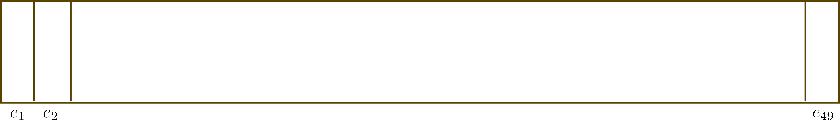
Here, we showcase only the positional encodings , , and each of dimension, a.k.a height 4.
Lets say, we wish to coach a Reformer model on sequences of a length of as much as 0.5M tokens and an input vector config.hidden_size of 1024 (see notebook here). The corresponding positional embeddings have a size of parameters, which corresponds to a size of 2GB.
Such positional encodings would use an unnecessarily great amount of memory each when loading the model in memory and when saving the model on a hard disk drive.
The Reformer authors managed to drastically shrink the positional encodings in size by cutting the config.hidden_size dimension in two and smartly factorizing
the dimension.
In Transformer, the user can resolve into which shape will be factorized into by setting config.axial_pos_shape to an appropriate
list of two values and in order that . By setting config.axial_pos_embds_dim to an
appropriate list of two values and in order that , the user can resolve how the hidden size dimension ought to be cut.
Now, let’s visualize and explain more intuitively.
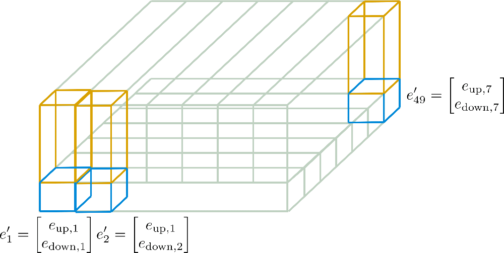
One can consider factorizing as folding the dimension right into a third axis, which is shown in the next for the factorization config.axial_pos_shape = [7, 7]:
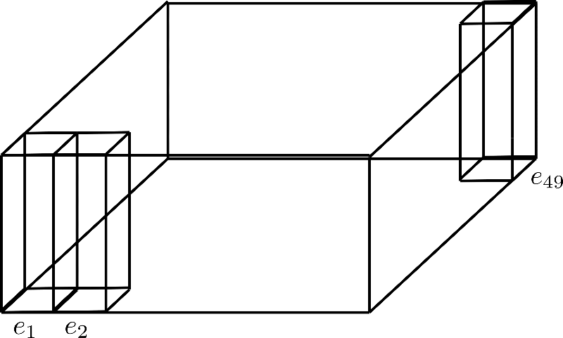
Each of the three standing rectangular prisms corresponds to one among the encoding vectors , but we will see that the 49 encoding vectors are divided into 7 rows of seven vectors each.
Now the thought is to make use of just one row of seven encoding vectors and expand those vectors to the opposite 6 rows, essentially reusing their values.
Since it is discouraged to have the identical values for various encoding vectors, each vector of dimension (a.k.a height) config.hidden_size=4 is cut into the lower encoding vector of size and of size , in order that the lower part will be expanded along the row dimension and the upper part will be expanded along the column dimension.
Let’s visualize for more clarity.
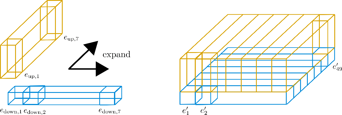
We will see that we’ve got cut the embedding vectors into (in blue) and (in yellow).
Now for the “sub”-vectors only the primary row, a.k.a. the width within the graphic, of is kept and expanded along the column dimension, a.k.a. the depth of the graphic. Inversely, for the “sub”-vectors only the primary column of is kept and expanded along the row dimension.
The resulting embedding vectors then correspond to
whereas and in our example.
These recent encodings are called Axial Position Encodings.
In the next, these axial position encodings are illustrated in additional detail for our example.
Now it ought to be more comprehensible how the ultimate positional encoding vectors are calculated only from of dimension and of dimension .
The crucial aspect to see here is that Axial Positional Encodings be sure that that not one of the vectors are equal to one another by design and that the general size of the encoding matrix is reduced from to .
By allowing each axial positional encoding vector to be different by design the model is given way more flexibility to learn efficient positional representations if axial positional encodings are learned by the model.
To exhibit the drastic reduction in size,
let’s assume we might have set config.axial_pos_shape = [1024, 512] and config.axial_pos_embds_dim = [512, 512] for a Reformer model that may process inputs as much as a length of 0.5M tokens. The resulting axial positional encoding matrix would have had a size of only parameters which corresponds to roughly 3MB. This can be a drastic reduction from the 2GB an ordinary positional encoding matrix would require on this case.
For a more condensed and math-heavy explanation please discuss with the 🤗Transformers docs here.
Benchmark
Lastly, let’s also compare the height memory consumption of conventional positional embeddings to axial positional embeddings.
#@title Installs and Imports
# pip installs
!pip -qq install git+https://github.com/huggingface/transformers.git
!pip install -qq py3nvml

from transformers import ReformerConfig, PyTorchBenchmark, PyTorchBenchmarkArguments, ReformerModel
Positional embeddings depend only on two configuration parameters: The utmost allowed length of input sequences config.max_position_embeddings and config.hidden_size. Let’s use a model that pushes the utmost allowed length of input sequences to half one million tokens, called google/reformer-crime-and-punishment, to see the effect of using axial positional embeddings.
To start with, we are going to compare the form of axial position encodings with standard positional encodings and the variety of parameters within the model.
config_no_pos_axial_embeds = ReformerConfig.from_pretrained("google/reformer-crime-and-punishment", axial_pos_embds=False)  # disable axial positional embeddings
config_pos_axial_embeds = ReformerConfig.from_pretrained("google/reformer-crime-and-punishment", axial_pos_embds=True, axial_pos_embds_dim=(64, 192), axial_pos_shape=(512, 1024))  # enable axial positional embeddings

print("Default Positional Encodings")
print(20 * '-')
model = ReformerModel(config_no_pos_axial_embeds)
print(f"Positional embeddings shape: {model.embeddings.position_embeddings}")
print(f"Num parameters of model: {model.num_parameters()}")
print(20 * '-' + 'nn')

print("Axial Positional Encodings")
print(20 * '-')
model = ReformerModel(config_pos_axial_embeds)
print(f"Positional embeddings shape: {model.embeddings.position_embeddings}")
print(f"Num parameters of model: {model.num_parameters()}")
print(20 * '-' + 'nn')
HBox(children=(FloatProgress(value=0.0, description='Downloading', max=1151.0, style=ProgressStyle(description…


Default Positional Encodings
--------------------
Positional embeddings shape: PositionEmbeddings(
  (embedding): Embedding(524288, 256)
)
Num parameters of model: 136572416
--------------------


Axial Positional Encodings
--------------------
Positional embeddings shape: AxialPositionEmbeddings(
  (weights): ParameterList(
      (0): Parameter containing: [torch.FloatTensor of size 512x1x64]
      (1): Parameter containing: [torch.FloatTensor of size 1x1024x192]
  )
)
Num parameters of model: 2584064
--------------------
Having read the idea, the form of the axial positional encoding weights shouldn’t be a surprise to the reader.
Regarding the outcomes, it may well be seen that for models being able to processing such long input sequences, it isn’t practical to make use of default positional encodings.
Within the case of google/reformer-crime-and-punishment, standard positional encodings alone contain greater than 100M parameters.
Axial positional encodings reduce this number to only over 200K.
Lastly, let’s also compare the required memory at inference time.
benchmark_args = PyTorchBenchmarkArguments(sequence_lengths=[512], batch_sizes=[8], models=["Reformer-No-Axial-Pos-Embeddings", "Reformer-Axial-Pos-Embeddings"], no_speed=True, no_env_print=True)
benchmark = PyTorchBenchmark(configs=[config_no_pos_axial_embeds, config_pos_axial_embeds], args=benchmark_args)
result = benchmark.run()
1 / 2
2 / 2

====================      INFERENCE - MEMORY - RESULT       ====================
--------------------------------------------------------------------------------
          Model Name             Batch Size     Seq Length    Memory in MB
--------------------------------------------------------------------------------
Reformer-No-Axial-Pos-Embeddin       8              512             959
Reformer-Axial-Pos-Embeddings        8              512             447
--------------------------------------------------------------------------------
It may be seen that using axial positional embeddings reduces the memory requirement to roughly half within the case of google/reformer-crime-and-punishment.