Scaling-up BERT Inference on CPU (Part 1)

Back in October 2019, my colleague Lysandre Debut published a comprehensive (on the time) inference performance
benchmarking blog (1).

Since then, 🤗 transformers (2) welcomed an amazing number
of recent architectures and hundreds of recent models were added to the 🤗 hub (3)
which now counts greater than 9,000 of them as of first quarter of 2021.

Because the NLP landscape keeps trending towards increasingly BERT-like models getting used in production, it
stays difficult to efficiently deploy and run these architectures at scale.
Because of this we recently introduced our 🤗 Inference API:
to allow you to concentrate on constructing value to your users and customers, relatively than digging into all of the highly
technical facets of running such models.

This blog post is the primary a part of a series which is able to cover many of the hardware and software optimizations to higher
leverage CPUs for BERT model inference.

For this initial blog post, we are going to cover the hardware part:

• Organising a baseline – Out of the box results
• Practical & technical considerations when leveraging modern CPUs for CPU-bound tasks
• Core count scaling – Does increasing the variety of cores actually give higher performance?
• Batch size scaling – Increasing throughput with multiple parallel & independent model instances

We decided to concentrate on essentially the most famous Transformer model architecture,
BERT (Delvin & al. 2018) (4). While we focus this blog post on BERT-like
models to maintain the article concise, all of the described techniques
may be applied to any architecture on the Hugging Face model hub.
On this blog post we is not going to describe intimately the Transformer architecture – to study that I can not
recommend enough the
Illustrated Transformer blogpost from Jay Alammar (5).

Today’s goals are to offer you an idea of where we’re from an Open Source perspective using BERT-like
models for inference on PyTorch and TensorFlow, and likewise what you may easily leverage to speedup inference.

2. Benchmarking methodology

With regards to leveraging BERT-like models from Hugging Face’s model hub, there are numerous knobs which might
be tuned to make things faster.
Also, as a way to quantify what “faster” means, we are going to depend on widely adopted metrics:

• Latency: Time it takes for a single execution of the model (i.e. forward call)
• Throughput: Variety of executions performed in a set period of time

These two metrics will help us understand the advantages and tradeoffs along this blog post.

The benchmarking methodology was reimplemented from scratch as a way to integrate the most recent features provided by transformers
and likewise to let the community run and share benchmarks in an hopefully easier way.
The entire framework is now based on Facebook AI & Research’s Hydra configuration library allowing us to simply report
and track all of the items involved while running the benchmark, hence increasing the general reproducibility.
Yow will discover the entire structure of the project here

On the 2021 version, we kept the flexibility to run inference workloads through PyTorch and Tensorflow as within the
previous blog (1) together with their traced counterpart
TorchScript (6), Google Accelerated Linear Algebra (XLA) (7).
Also, we decided to incorporate support for ONNX Runtime (8) because it provides many optimizations
specifically targeting transformers based models which makes it a powerful candidate to contemplate when discussing
performance.

Last but not least, this latest unified benchmarking environment will allow us to simply run inference for various scenarios
reminiscent of Quantized Models (Zafrir & al.) (9)
using less precise number representations (float16, int8, int4).
This method often called quantization has seen an increased adoption amongst all major hardware providers.
Within the near future, we would love to integrate additional methods we’re actively working on at Hugging Face, namely Distillation, Pruning & Sparsificaton.

3. Baselines

All the outcomes below were run on Amazon Web Services (AWS) c5.metal instance
leveraging an Intel Xeon Platinum 8275 CPU (48 cores/96 threads).
The alternative of this instance provides all of the useful CPU features to speedup Deep Learning workloads reminiscent of:

• AVX512 instructions set (which could not be leveraged out-of-the-box by the assorted frameworks)
• Intel Deep Learning Boost (also often called Vector Neural Network Instruction – VNNI) which provides specialized
  CPU instructions for running quantized networks (using int8 data type)

The alternative of using metal instance is to avoid any virtualization issue which might arise when using cloud providers.
This offers us full control of the hardware, especially while targeting the NUMA (Non-Unified Memory Architecture) controller, which
we are going to cover later on this post.

The operating system was Ubuntu 20.04 (LTS) and all of the experiments were conducted using Hugging Face transformers version 4.5.0, PyTorch 1.8.1 & Google TensorFlow 2.4.0

4. Out of the box results

Straigh to the purpose, out-of-the-box, PyTorch shows higher inference results over TensorFlow for all of the configurations tested here.
It can be crucial to notice the outcomes out-of-the-box won’t reflect the “optimal” setup for each PyTorch and TensorFlow and thus it could possibly look deceiving here.

One possible approach to explain such difference between the 2 frameworks is perhaps the underlying technology to
execute parallel sections inside operators.
PyTorch internally uses OpenMP (10) together with Intel MKL (now oneDNN) (11) for efficient linear algebra computations whereas TensorFlow relies on Eigen and its own threading implementation.

5. Scaling BERT Inference to extend overall throughput on modern CPU

5.1. Introduction

There are multiple ways to enhance the latency and throughput for tasks reminiscent of BERT inference.
Improvements and tuning may be performed at various levels from enabling Operating System features, swapping dependent
libraries with more performant ones, rigorously tuning framework properties and, last but not least,
using parallelization logic leveraging all of the cores on the CPU(s).

For the rest of this blog post we are going to concentrate on the latter, also often called Multiple Inference Stream.

The thought is easy: Allocate multiple instances of the identical model and assign the execution of every instance to a
dedicated, non-overlapping subset of the CPU cores as a way to have truly parallel instances.

5.2. Cores and Threads on Modern CPUs

On our way towards optimizing CPU inference for higher usage of the CPU cores you may have already seen –at the least for the
past 20 years– modern CPUs specifications report “cores” and “hardware threads” or “physical” and “logical” numbers.
These notions seek advice from a mechanism called Simultaneous Multi-Threading (SMT) or Hyper-Threading on Intel’s platforms.

As an example this, imagine two tasks A and B, executing in parallel, each by itself software thread.
Sooner or later, there may be a high probability these two tasks may have to attend for some resources to be fetched from essential memory, SSD, HDD
and even the network.
If the threads are scheduled on different physical cores, with no hyper-threading,
during these periods the core executing the duty is in an Idle state waiting for the resources to reach, and effectively doing nothing… and hence not getting fully utilized

Now, with SMT, the two software threads for task A and B may be scheduled on the identical physical core,
such that their execution is interleaved on that physical core:

Task A and Task B will execute concurrently on the physical core and when one task is halted, the opposite task can still proceed execution
on the core thereby increasing the utilization of that core.

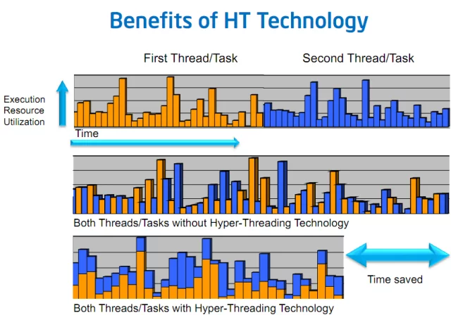
The figure 3. above simplifies the situation by assuming single core setup. For those who want some more details on how SMT works on multi-cores CPUs, please
seek advice from these two articles with very deep technical explanations of the behavior:

Back to our model inference workload… For those who give it some thought, in an ideal world with a completely optimized setup, computations take nearly all of time.
On this context, using the logical cores shouldn’t bring us any performance profit because each logical cores (hardware threads) compete for the core’s execution resources.
Because of this, the tasks being a majority of general matrix multiplications (gemms (14)), they’re inherently CPU bounds and doesn’t advantages from SMT.

5.3. Leveraging Multi-Socket servers and CPU affinity

Nowadays servers bring many cores, a few of them even support multi-socket setups (i.e. multiple CPUs on the motherboard).
On Linux, the command lscpu reports all of the specifications and topology of the CPUs present on the system:

ubuntu@some-ec2-machine:~$ lscpu
Architecture:                    x86_64
CPU op-mode(s):                  32-bit, 64-bit
Byte Order:                      Little Endian
Address sizes:                   46 bits physical, 48 bits virtual
CPU(s):                          96
On-line CPU(s) list:             0-95
Thread(s) per core:              2
Core(s) per socket:              24
Socket(s):                       2
NUMA node(s):                    2
Vendor ID:                       GenuineIntel
CPU family:                      6
Model:                           85
Model name:                      Intel(R) Xeon(R) Platinum 8275CL CPU @ 3.00GHz
Stepping:                        7
CPU MHz:                         1200.577
CPU max MHz:                     3900.0000
CPU min MHz:                     1200.0000
BogoMIPS:                        6000.00
Virtualization:                  VT-x
L1d cache:                       1.5 MiB
L1i cache:                       1.5 MiB
L2 cache:                        48 MiB
L3 cache:                        71.5 MiB
NUMA node0 CPU(s):               0-23,48-71
NUMA node1 CPU(s):               24-47,72-95

In our case we have now a machine with 2 sockets, each socket providing 24 physical cores with 2 threads per cores (SMT).
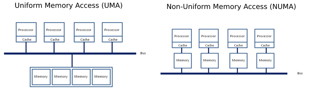
One other interesting characteristic is the notion of NUMA node (0, 1) which represents how cores and memory are being
mapped on the system.

Non-Uniform Memory Access (NUMA) is the alternative of Uniform Memory Access (UMA) where the entire memory pool
is accessible by all of the cores through a single unified bus between sockets and the essential memory.
NUMA then again splits the memory pool and every CPU socket is responsible to deal with a subset of the memory,
reducing the congestion on the bus.

With a view to fully utilize the potential of such a beefy machine, we want to make sure our model instances are accurately
dispatched across all of the physical cores on all sockets together with enforcing memory allocation to be “NUMA-aware”.

On Linux, NUMA’s process configuration may be tuned through numactl which provides an interface to bind a process to a
set of CPU cores (referred as Thread Affinity).
Also, it allows tuning the memory allocation policy, ensuring the memory allocated for the method
is as close as possible to the cores’ memory pool (referred as Explicit Memory Allocation Directives).

Note: Setting each cores and memory affinities is significant here. Having computations done on socket 0 and memory allocated
on socket 1 would ask the system to go over the sockets shared bus to exchange memory, thus resulting in an undesired overhead.

5.4. Tuning Thread Affinity & Memory Allocation Policy

Now that we have now all of the knobs required to regulate the resources’ allocation of our model instances we go further and see
effectively deploy those and see the impact on latency and throughput.
Let’s go steadily to get a way of what’s the impact of every command and parameter.

First, we start by launching our inference model with none tuning, and we observe how the computations are being dispatched on CPU cores (Left).

python3 src/essential.py model=bert-base-cased backend.name=pytorch batch_size=1 sequence_length=128

Then we specify the core and memory affinity through numactl using all of the physical cores and only a single thread (thread 0) per core (Right):

numactl -C 0-47 -m 0,1 python3 src/essential.py model=bert-base-cased backend.name=pytorch batch_size=1 sequence_length=128

As you may see, with none specific tuning, PyTorch and TensorFlow dispatch the work on a single socket, using all of the logical cores in that socket (each threads on 24 cores).
Also, as we highlighted earlier, we are not looking for to leverage the SMT feature in our case, so we set the method’ thread affinity to focus on only one hardware thread.

Note, this is restricted to this run and may vary depending on individual setups. Hence, it is suggested to ascertain thread affinity settings for every specific use-case.

Let’s take sometime from here to focus on what we did with numactl:

• -C 0-47 indicates to numactl what’s the thread affinity (cores 0 to 47).
• -m 0,1 indicates to numactl to allocate memory on each CPU sockets

For those who wonder why we’re binding the method to cores [0…47], it’s worthwhile to return to have a look at the output of lscpu.
From there you will see the section NUMA node0 and NUMA node1 which has the shape NUMA node

In our case, each socket is one NUMA node and there are 2 NUMA nodes.
Each socket or each NUMA node has 24 physical cores and a couple of hardware threads per core, so 48 logical cores.
For NUMA node 0, 0-23 are hardware thread 0 and 24-47 are hardware thread 1 on the 24 physical cores in socket 0.
Likewise, for NUMA node 1, 48-71 are hardware thread 0 and 72-95 are hardware thread 1 on the 24 physical cores in socket 1.

As we’re targeting just 1 thread per physical core, as explained earlier, we pick only thread 0 on each core and hence logical processors 0-47.
Since we’re using each sockets, we want to also bind the memory allocations accordingly (0,1).

Please note that using each sockets may not at all times give the very best results, particularly for small problem sizes.
The advantage of using compute resources across each sockets is perhaps reduced and even negated by cross-socket communication overhead.

6. Core count scaling – Does using more cores actually improve performance?

When fascinated with possible ways to enhance our model inference performances, the primary rational solution is perhaps to
throw some more resources to do the identical amount of labor.
Through the remainder of this blog series, we are going to seek advice from this setup as Core Count Scaling meaning, only the number
of cores used on the system to realize the duty will vary. This can also be often referred as Strong Scaling within the HPC world.

At this stage, you could wonder what’s the point of allocating only a subset of the cores relatively than throwing
all of the horses at the duty to realize minimum latency.

Indeed, depending on the problem-size, throwing more resources to the duty might give higher results.
Additionally it is possible that for small problems putting more CPU cores at work doesn’t improve the ultimate latency.

With a view to illustrate this, the figure 6. below takes different problem sizes (batch_size = 1, sequence length = {32, 128, 512})
and reports the latencies with respect to the variety of CPU cores used for running
computations for each PyTorch and TensorFlow.

Limiting the variety of resources involved in computation is finished by limiting the CPU cores involved in
intra operations (intra here means inside an operator doing computation, also often called “kernel”).

That is achieved through the next APIs:

• PyTorch: torch.set_num_threads(x)
• TensorFlow: tf.config.threading.set_intra_op_parallelism_threads(x)

As you may see, depending on the issue size, the variety of threads involved within the computations has a positive impact
on the latency measurements.

For small-sized problems & medium-sized problems using just one socket would give the very best performance.
For big-sized problems, the overhead of the cross-socket communication is roofed by the computations cost, thus benefiting from
using all of the cores available on the each sockets.

7. Multi-Stream Inference – Using multiple instances in parallel

For those who’re still reading this, you must now be in good condition to establish parallel inference workloads on CPU.
Now, we’re going to focus on some possibilities offered by the powerful hardware we have now, and tuning the knobs described before,
to scale our inference as linearly as possible.

In the next section we are going to explore one other possible scaling solution Batch Size Scaling, but before diving into this, let’s
take a take a look at how we are able to leverage Linux tools as a way to assign Thread Affinity allowing effective model instance parallelism.

As an alternative of throwing more cores to the duty as you’d do within the core count scaling setup, now we can be using more model instances.
Each instance will run independently by itself subset of the hardware resources in a very parallel fashion on a subset of the CPU cores.

7.1. How-to allocate multiple independent instances

Let’s start easy, if we would like to spawn 2 instances, one on each socket with 24 cores assigned:

numactl -C 0-23 -m 0 python3 src/essential.py model=bert-base-cased batch_size=1 sequence_length=128 backend.name=pytorch backend.num_threads=24
numactl -C 24-47 -m 1 python3 src/essential.py model=bert-base-cased batch_size=1 sequence_length=128 backend.name=pytorch backend.num_threads=24

Ranging from here, each instance doesn’t share any resource with the opposite, and every part is working at maximum efficiency from a
hardware perspective.
The latency measurements are similar to what a single instance would achieve, but throughput is definitely 2x higher
because the two instances operate in a very parallel way.

We are able to further increase the variety of instances, lowering the variety of cores assigned for every instance.
Let’s run 4 independent instances, each of them effectively sure to 12 CPU cores.

numactl -C 0-11 -m 0 python3 src/essential.py model=bert-base-cased batch_size=1 sequence_length=128 backend.name=pytorch backend.num_threads=12
numactl -C 12-23 -m 0 python3 src/essential.py model=bert-base-cased batch_size=1 sequence_length=128 backend.name=pytorch backend.num_threads=12
numactl -C 24-35 -m 1 python3 src/essential.py model=bert-base-cased batch_size=1 sequence_length=128 backend.name=pytorch backend.num_threads=12
numactl -C 36-47 -m 1 python3 src/essential.py model=bert-base-cased batch_size=1 sequence_length=128 backend.name=pytorch backend.num_threads=12

The outcomes remain the identical, our 4 instances are effectively running in a very parallel manner.
The latency can be barely higher than the instance before (2x less cores getting used), however the throughput can be again 2x higher.

7.2. Smart dispatching – Allocating different model instances for various problem sizes

Each other possibility offered by this setup is to have multiple instances rigorously tuned for various problem sizes.
With a sensible dispatching approach, one can redirect incoming requests to the proper configuration giving the very best latency depending on the request workload.

# Small-sized problems (sequence length <= 32) use only 8 cores (on socket 0 - 8/24 cores used)
numactl -C 0-7 -m 0 python3 src/essential.py model=bert-base-cased batch_size=1 sequence_length=32 backend.name=pytorch backend.num_threads=8

# Medium-sized problems (32 > sequence <= 384) use remaining 16 cores (on socket 0 - (8+16)/24 cores used)
numactl -C 8-23 -m 0 python3 src/essential.py model=bert-base-cased batch_size=1 sequence_length=128 backend.name=pytorch backend.num_threads=16

# Large sized problems (sequence >= 384) use all the CPU (on socket 1 - 24/24 cores used)
numactl -C 24-37 -m 1 python3 src/essential.py model=bert-base-cased batch_size=1 sequence_length=384 backend.name=pytorch backend.num_threads=24

8. Batch size scaling – Improving throughput and latency with multiple parallel & independent model instances

Each other very interesting direction for scaling up inference is to truly put some more model instances into the pool
together with reducing the actual workload each instance receives proportionally.

This method actually changes each the dimensions of the issue (batch size), and the resources involved within the computation (cores).

As an example, imagine you may have a server with C CPU cores, and you need to run a workload containing B samples with S tokens.
You may represent this workload as a tensor of shape [B, S], B being the dimensions of the batch and S being the utmost sequence length throughout the B samples.

For all of the instances (N), each of them executes on C / N cores and would receive a subset of the duty [B / N, S].

Each instance doesn’t receive the worldwide batch but as an alternative, all of them receive a subset of it [B / N, S] thus the name Batch Size Scaling.
With a view to highlight the advantages of such scaling method, the charts below reports each the latencies when scaling up model instances together with the results on the throughput.

When taking a look at the outcomes, let’s concentrate on the latency and the throughput facets:

On one hand, we’re taking the utmost latency over the pool of instances to reflect the time it takes to process all of the samples within the batch.
Putting it in another way, as instances operate in a very parallel fashion, the time it takes to assemble all of the batch chunks from all of the instances
is driven by the longest time it takes for individual instance within the pool to get their chunk done.

As you may see below on Figure 7., the actual latency gain when increasing the variety of instances is admittedly dependent of the issue size.
In all cases, we are able to find an optimal resource allocation (batch size & variety of instances) to reduce our latency but, there is no such thing as a specific pattern on the variety of cores to involve within the computation.

Also, it can be crucial to note the outcomes might look totally different on one other system (i.e. Operating System, Kernel Version, Framework version, etc.)

Figure 8. sums up the very best multi-instance configuration when targeting minimum latency by taking the minimum over the variety of instances involved.
For example, for {batch = 8, sequence length = 128} using 4 instances (each with {batch = 2} and 12 cores) gives the very best latency measurements.

The Figure 9. reports all of the setups minimizing latency for each PyTorch and TensorFlow for various problem-sizes.

Spoiler: There are many other optimizations we are going to discuss in a follow-up blog post which is able to substantially impact this chart.

On a second hand, we observe the throughput because the sum of all of the model instance executing in parallel.
It allows us to visualise the scalability of the system when adding increasingly instances each of them with fewer resources but in addition proportional workload.
Here, the outcomes show almost linear scalability and thus an optimal hardware usage.

9. Conclusion

Through this blog post, we covered out-of-box BERT inference performance one can expect for PyTorch and TensorFlow,
from an easy PyPi install and without further tuning.
It can be crucial to focus on results provided here reflects out-of-the-box framework setup hence, they may not provide the very best performances.
We decided to not include optimizations as a part of this blog post to concentrate on hardware and efficiency.
Optimizations can be discussed within the second part! 🚀

Then, we covered and detailed the impact, and the importance of setting the thread affinity together with the trade-off between the goal problem size, and the variety of cores required for achieving the duty.
Also, it can be crucial to define which criteria (i.e. latency vs throughput) to make use of when optimizing your deployment because the resulting setups is perhaps totally different.

On a more general note, small problem sizes (short sequences and/or small batches) might require much fewer cores to realize the very best possible latency than big problems (very long sequences and/or big batches).

It’s interesting to cover all these facets when fascinated with the ultimate deployment platform as it’d cut the price of the infrastructure drastically.
For example, our 48 cores machine charges 4.848$/h whereas a smaller instances with only 8 cores lowers the price to 0.808$/h, resulting in a 6x cost reduction.

Last but not least, lots of the knobs discussed along this blog post may be robotically tuned through a launcher script
highly inspired from the unique script made by Intel and available here.
The launcher script is capable of robotically starts your python process(es) with the right thread affinity, effectively
splitting resources across instances together with many other performances suggestions! We’ll detail a lot of this suggestions within the second part 🧐.

Within the follow-up blog post, more advanced settings and tuning techniques to diminish model latency even further can be involved, reminiscent of:

• Launcher script walk-through
• Tuning the memory allocation library
• Using Linux’s Transparent Huge Pages mechanisms
• Using vendor-specific Math/Parallel libraries

Stay tuned! 🤗

Acknowledgments

• Omry Yadan (Facebook FAIR) – Writer of OmegaConf & Hydra for all the guidelines organising Hydra accurately.
• All Intel & Intel Labs’ NLP colleagues – For the continued optimizations and research efforts they’re putting into transformers and more generally within the NLP field.
• Hugging Face colleagues – For all of the comments and enhancements within the reviewing process.

References

1. Benchmarking Transformers: PyTorch and TensorFlow
2. HuggingFace’s Transformers: State-of-the-art Natural Language Processing
3. HuggingFace’s Model Hub
4. BERT – Pre-training of Deep Bidirectional Transformers for Language Understanding (Devlin & al. 2018)
5. Illustrated Transformer blogpost from Jay Alammar
6. PyTorch – TorchScript
7. Google Accelerated Linear Algebra (XLA)
8. ONNX Runtime – Optimize and Speed up Machine Learning Inferencing and Training
9. Q8BERT – Quantized 8Bit BERT (Zafrir & al. 2019)
10. OpenMP
11. Intel oneDNN
12. Intel® Hyper-Threading Technology – Technical User Guide
13. Introduction to Hyper-Threading Technology
14. BLAS (Basic Linear Algebra Subprogram) – Wikipedia
15. Optimizing Applications for NUMA