An Introduction to Q-Learning Part 1

⚠️ A recent updated version of this text is obtainable here 👉 https://huggingface.co/deep-rl-course/unit1/introduction

This text is an element of the Deep Reinforcement Learning Class. A free course from beginner to expert. Check the syllabus here.

⚠️ A recent updated version of this text is obtainable here 👉 https://huggingface.co/deep-rl-course/unit1/introduction

This text is an element of the Deep Reinforcement Learning Class. A free course from beginner to expert. Check the syllabus here.

Within the first chapter of this class, we learned about Reinforcement Learning (RL), the RL process, and the various methods to unravel an RL problem. We also trained our first lander agent to land appropriately on the Moon 🌕 and uploaded it to the Hugging Face Hub.

So today, we will dive deeper into one in every of the Reinforcement Learning methods: value-based methods and study our first RL algorithm: Q-Learning.

We’ll also implement our first RL agent from scratch: a Q-Learning agent and can train it in two environments:

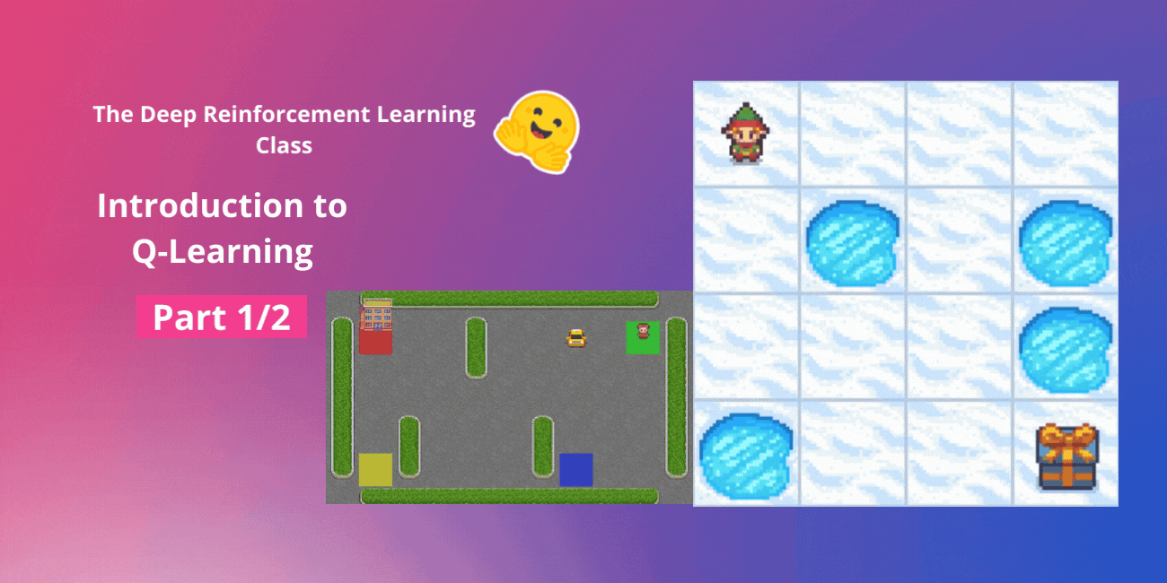
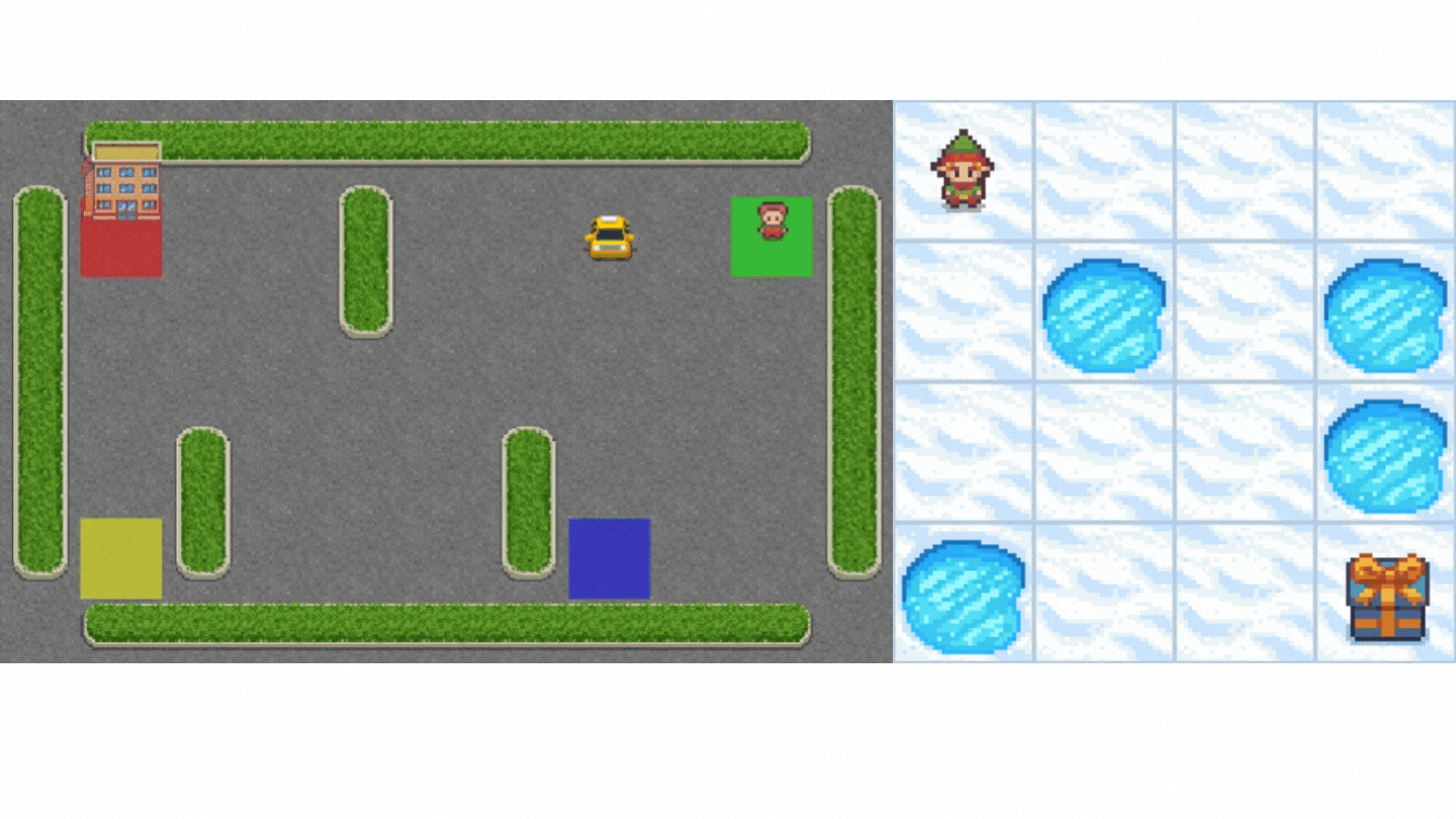
1. Frozen-Lake-v1 (non-slippery version): where our agent might want to go from the starting state (S) to the goal state (G) by walking only on frozen tiles (F) and avoiding holes (H).
2. An autonomous taxi will need to learn to navigate a city to transport its passengers from point A to point B.

This unit is split into 2 parts:

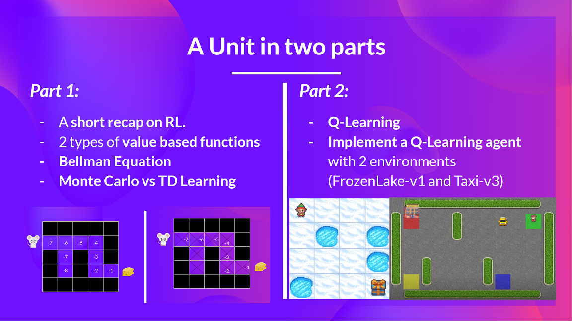
In the primary part, we’ll learn concerning the value-based methods and the difference between Monte Carlo and Temporal Difference Learning.

And within the second part, we’ll study our first RL algorithm: Q-Learning, and implement our first RL Agent.

This unit is key if you wish to have the option to work on Deep Q-Learning (unit 3): the primary Deep RL algorithm that was in a position to play Atari games and beat the human level on a few of them (breakout, space invaders…).

So let’s start!

What’s RL? A brief recap

In RL, we construct an agent that may make smart decisions. As an illustration, an agent that learns to play a video game. Or a trading agent that learns to maximise its advantages by making smart decisions on what stocks to purchase and when to sell.

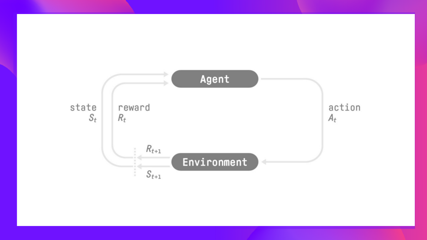
But, to make intelligent decisions, our agent will learn from the environment by interacting with it through trial and error and receiving rewards (positive or negative) as unique feedback.

Its goal is to maximise its expected cumulative reward (due to reward hypothesis).

The agent’s decision-making process is known as the policy π: given a state, a policy will output an motion or a probability distribution over actions. That’s, given an statement of the environment, a policy will provide an motion (or multiple probabilities for every motion) that the agent should take.

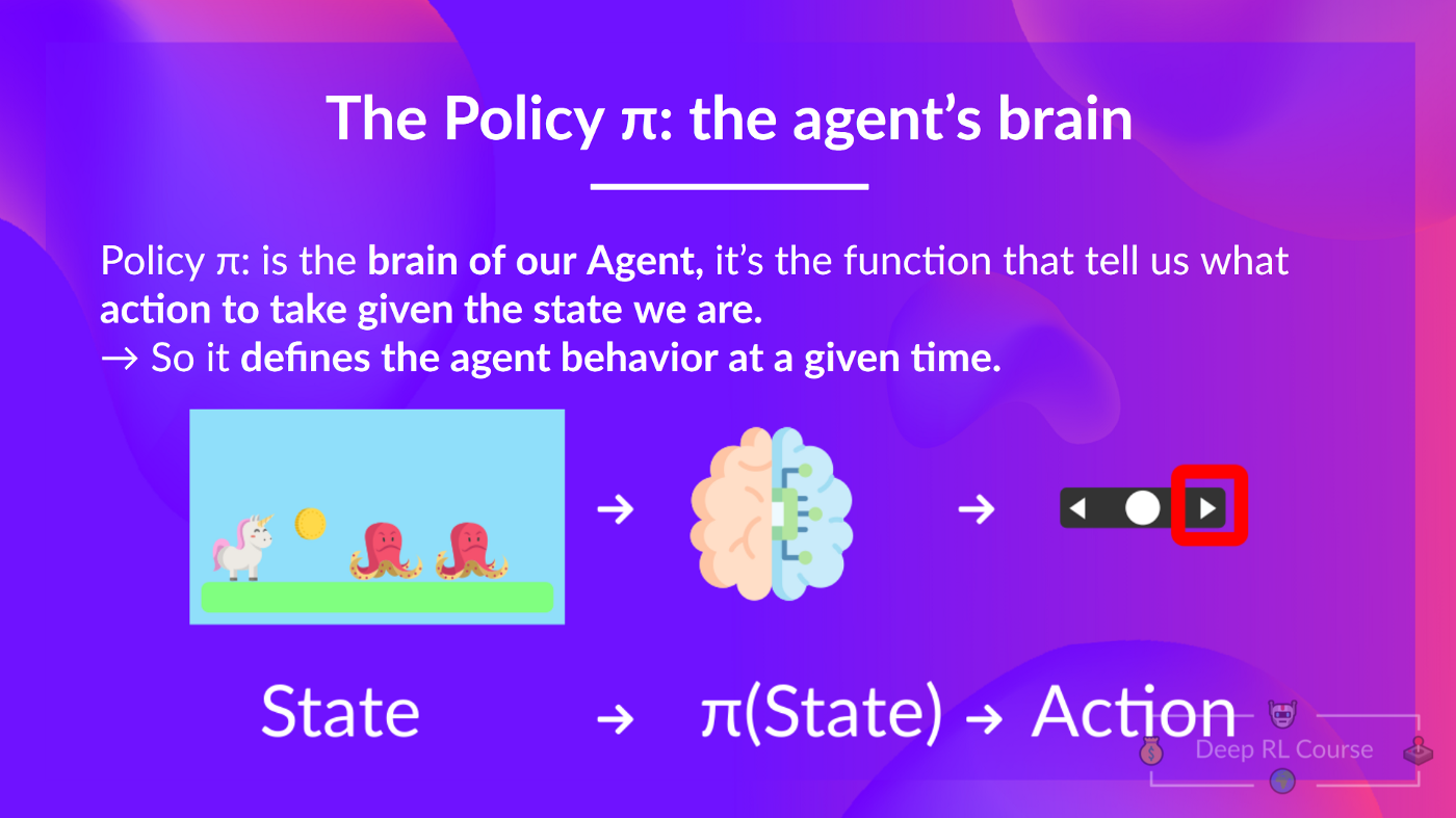
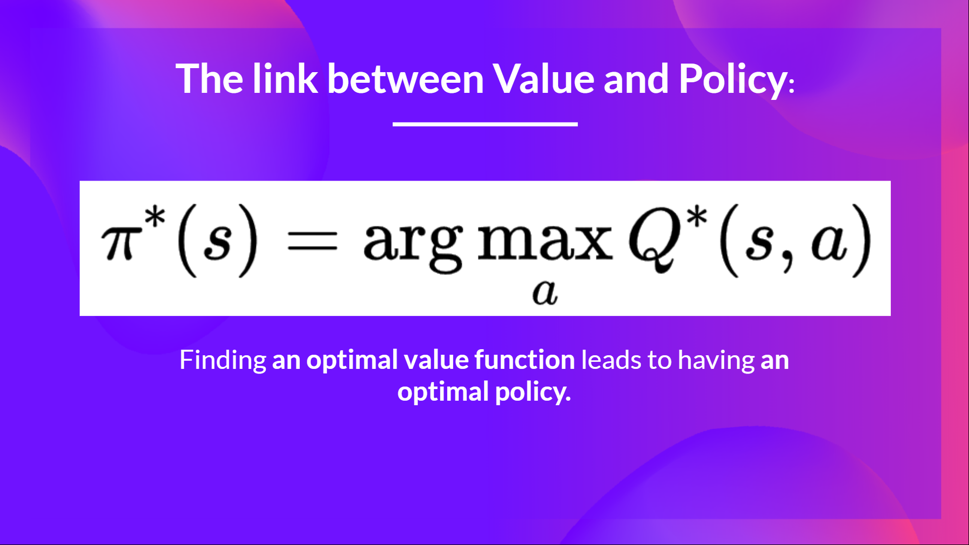
Our goal is to search out an optimal policy π*, aka., a policy that results in the most effective expected cumulative reward.

And to search out this optimal policy (hence solving the RL problem), there are two most important kinds of RL methods:

• Policy-based methods: Train the policy directly to learn which motion to take given a state.
• Value-based methods: Train a price function to learn which state is more beneficial and use this value function to take the motion that results in it.

And on this chapter, we’ll dive deeper into the Value-based methods.

The 2 kinds of value-based methods

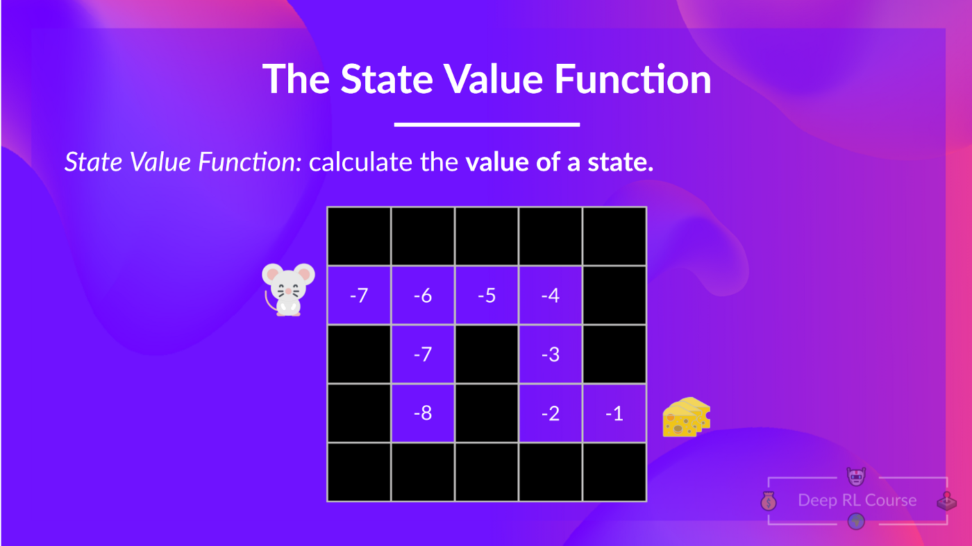
In value-based methods, we learn a price function that maps a state to the expected value of being at that state.

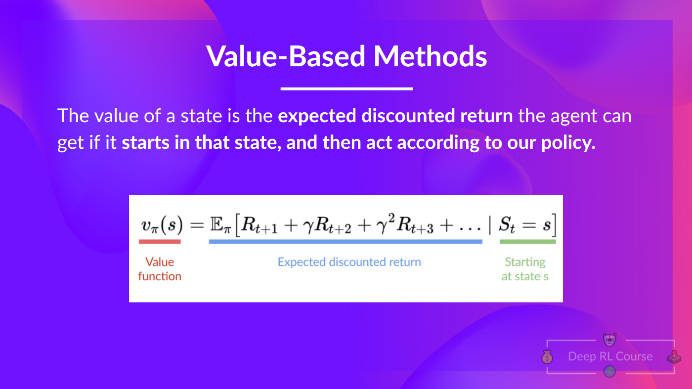
The worth of a state is the expected discounted return the agent can get if it starts at that state after which acts based on our policy.

In the event you forgot what discounting is, you can read this section.

But what does it mean to act based on our policy? In spite of everything, we do not have a policy in value-based methods, since we train a price function and never a policy.

Keep in mind that the goal of an RL agent is to have an optimal policy π.

To search out it, we learned that there are two different methods:

• Policy-based methods: Directly train the policy to pick what motion to take given a state (or a probability distribution over actions at that state). On this case, we do not have a price function.

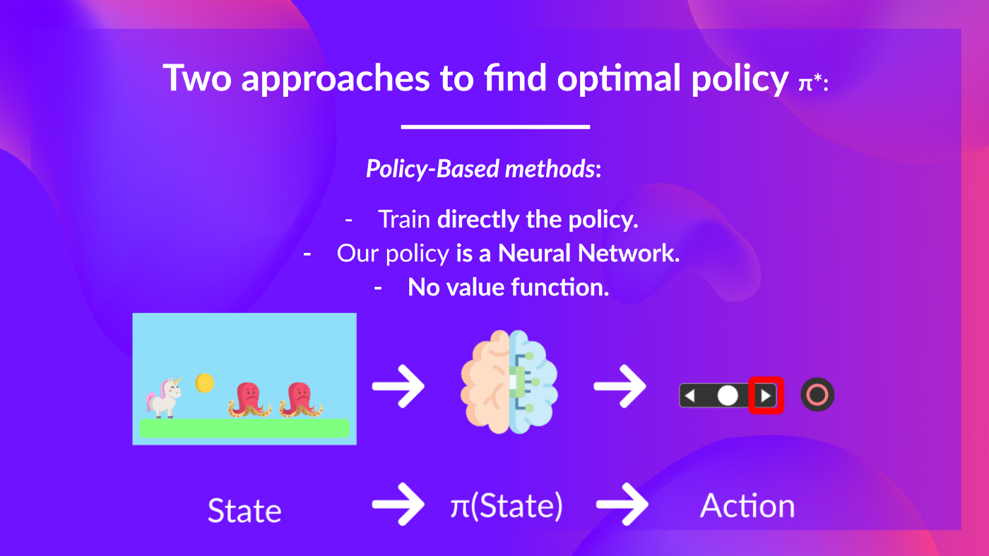
The policy takes a state as input and outputs what motion to take at that state (deterministic policy).

And consequently, we do not define by hand the behavior of our policy; it is the training that may define it.

• Value-based methods: Not directly, by training a price function that outputs the worth of a state or a state-action pair. Given this value function, our policy will take motion.

But, because we didn’t train our policy, we’d like to specify its behavior. As an illustration, if we wish a policy that, given the worth function, will take actions that at all times result in the most important reward, we’ll create a Greedy Policy.

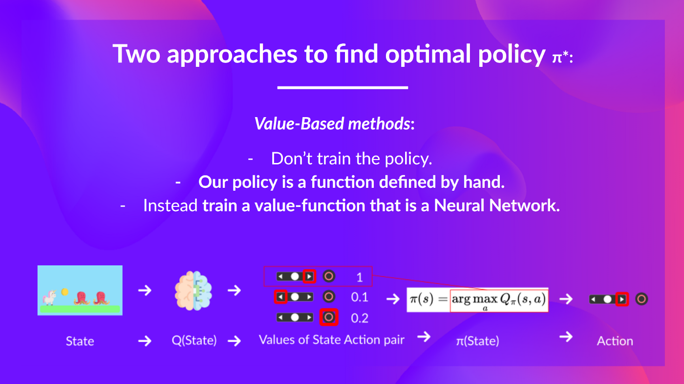
Consequently, whatever method you utilize to unravel your problem, you’ll have a policy, but within the case of value-based methods you do not train it, your policy is just a straightforward function that you just specify (as an example greedy policy) and this policy uses the values given by the value-function to pick its actions.

So the difference is:

• In policy-based, the optimal policy is found by training the policy directly.
• In value-based, finding an optimal value function results in having an optimal policy.

Actually, more often than not, in value-based methods, you may use an Epsilon-Greedy Policy that handles the exploration/exploitation trade-off; we’ll discuss it after we discuss Q-Learning within the second a part of this unit.

So, we have now two kinds of value-based functions:

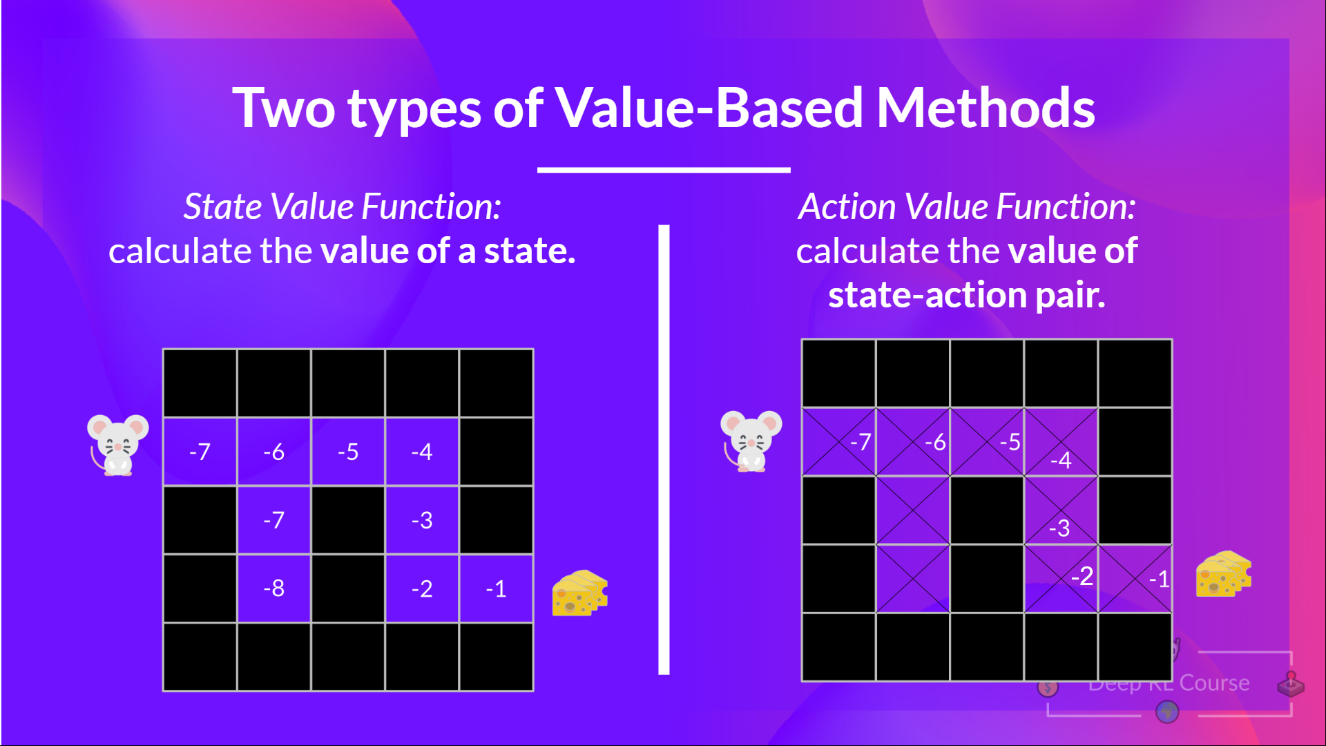
The State-Value function

We write the state value function under a policy π like this:

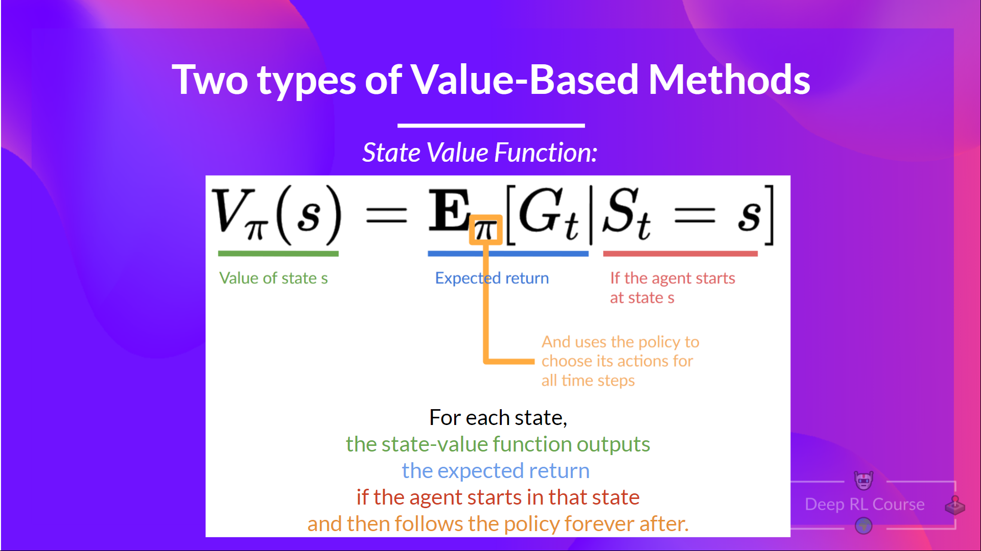
For every state, the state-value function outputs the expected return if the agent starts at that state, after which follow the policy eternally after (for all future timesteps when you prefer).

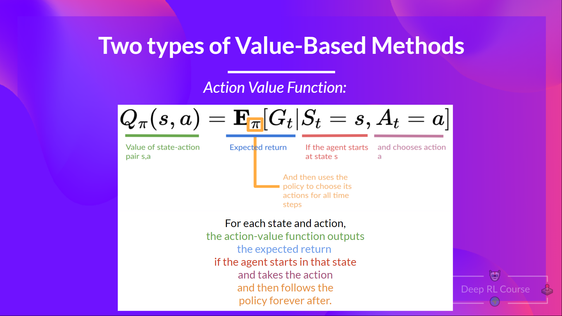
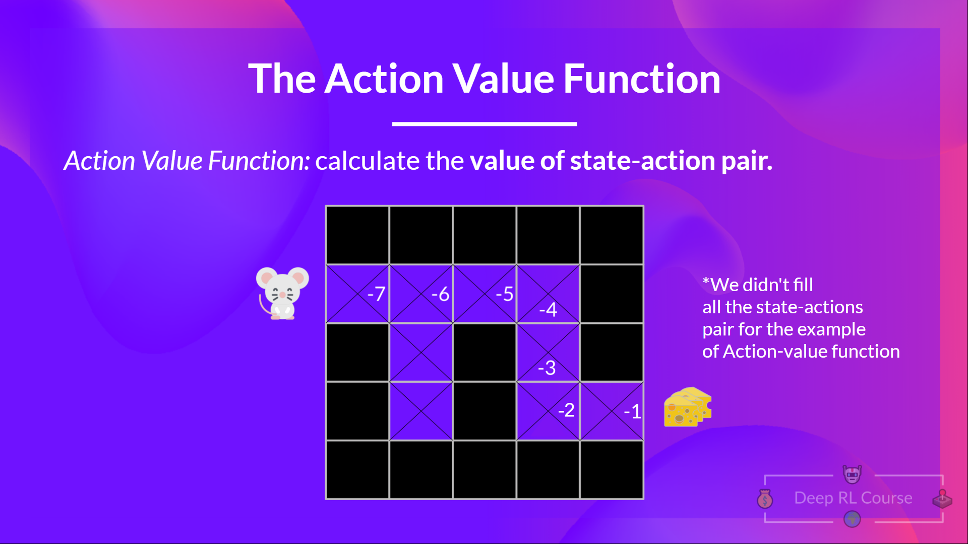
The Motion-Value function

Within the Motion-value function, for every state and motion pair, the action-value function outputs the expected return if the agent starts in that state and takes motion, after which follows the policy eternally after.

The worth of taking motion an in state s under a policy π is:

We see that the difference is:

• In state-value function, we calculate the worth of a state $S_{t}S\_t$
• In action-value function, we calculate the worth of the state-action pair ( $S_t,A_{t}S\_t,\; A\_t$

In either case, whatever value function we decide (state-value or action-value function), the worth is the expected return.

Nonetheless, the issue is that it implies that to calculate EACH value of a state or a state-action pair, we’d like to sum all of the rewards an agent can get if it starts at that state.

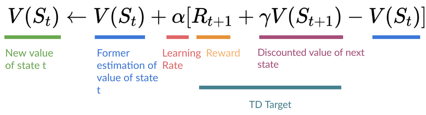
This could be a tedious process, and that is where the Bellman equation comes to assist us.

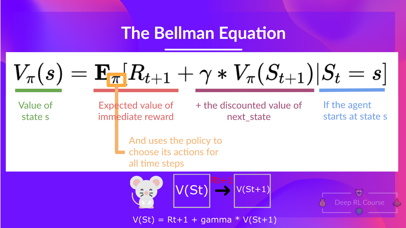
The Bellman Equation: simplify our worth estimation

The Bellman equation simplifies our state value or state-action value calculation.

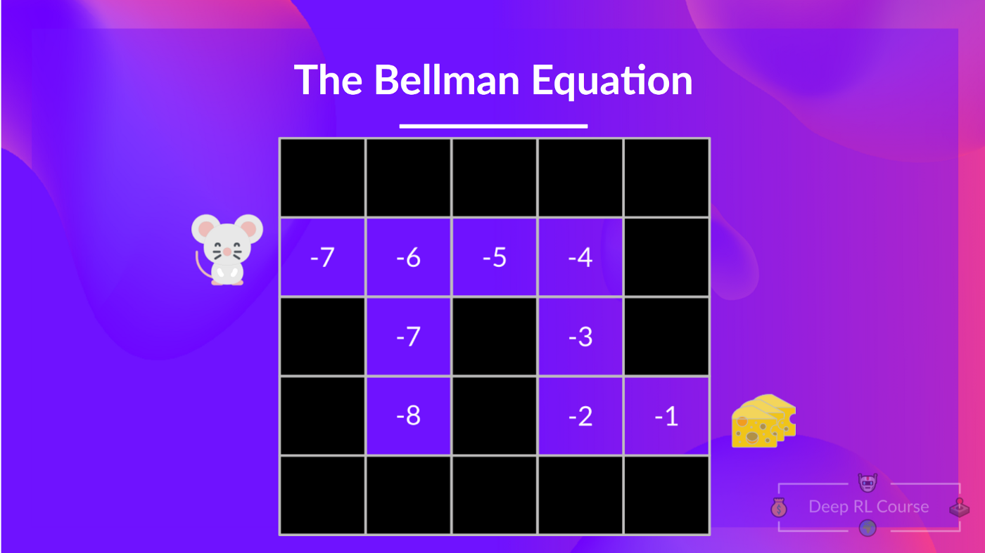
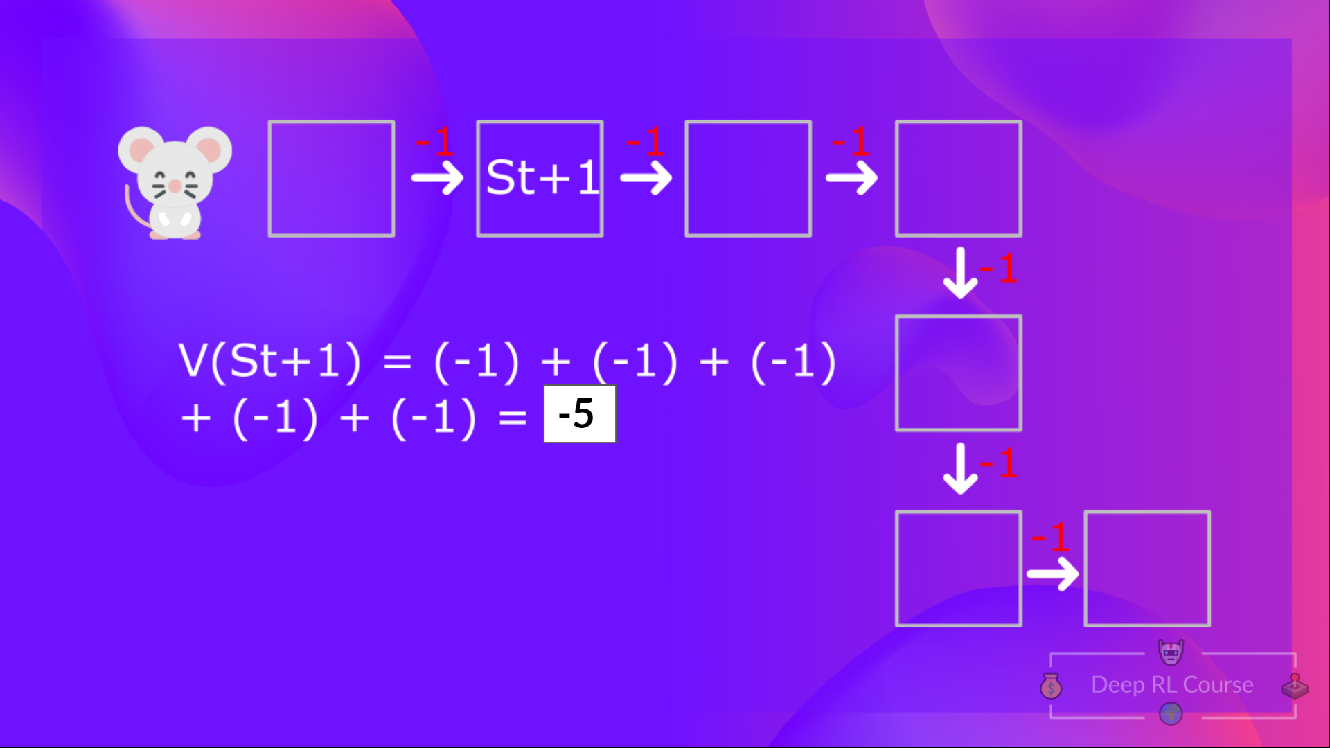
With what we learned from now, we all know that if we calculate the $V(S_t)V(S\_t)$

So to calculate $V(S_t)V(S\_t)$

Then, to calculate the $V(S_{t+1})V(S\_\{t+1\})$

So that you see, that is a reasonably tedious process if you’ll want to do it for every state value or state-action value.

As a substitute of calculating the expected return for every state or each state-action pair, we are able to use the Bellman equation.

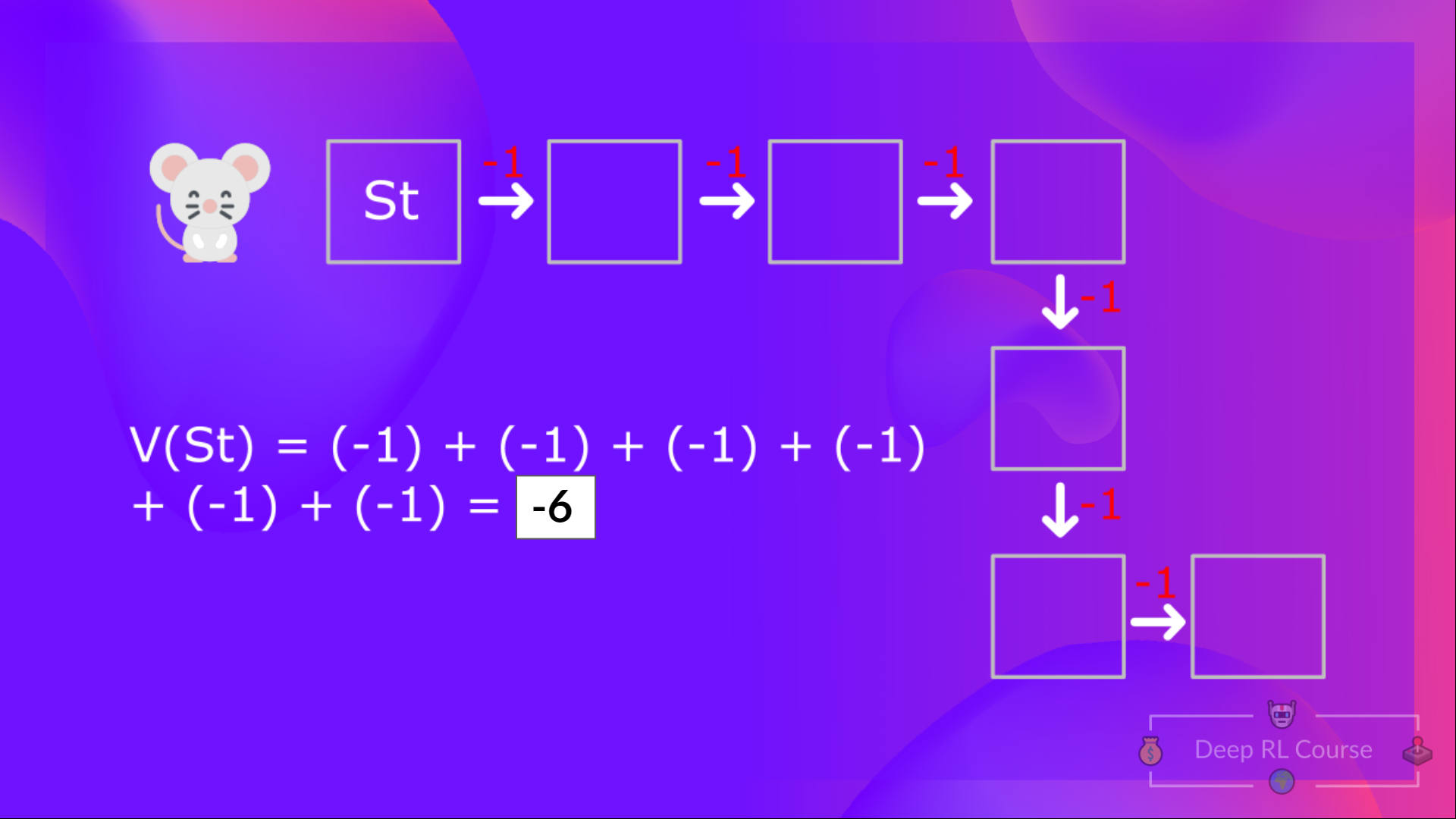
The Bellman equation is a recursive equation that works like this: as a substitute of starting for every state from the start and calculating the return, we are able to consider the worth of any state as:

The immediate reward $R_{t+1}R\_\{t+1\}$

If we return to our example, the worth of State 1= expected cumulative return if we start at that state.

To calculate the worth of State 1: the sum of rewards if the agent began in that state 1 after which followed the policy for on a regular basis steps.

Which is comparable to $V(S_t)V(S\_\{t\})$

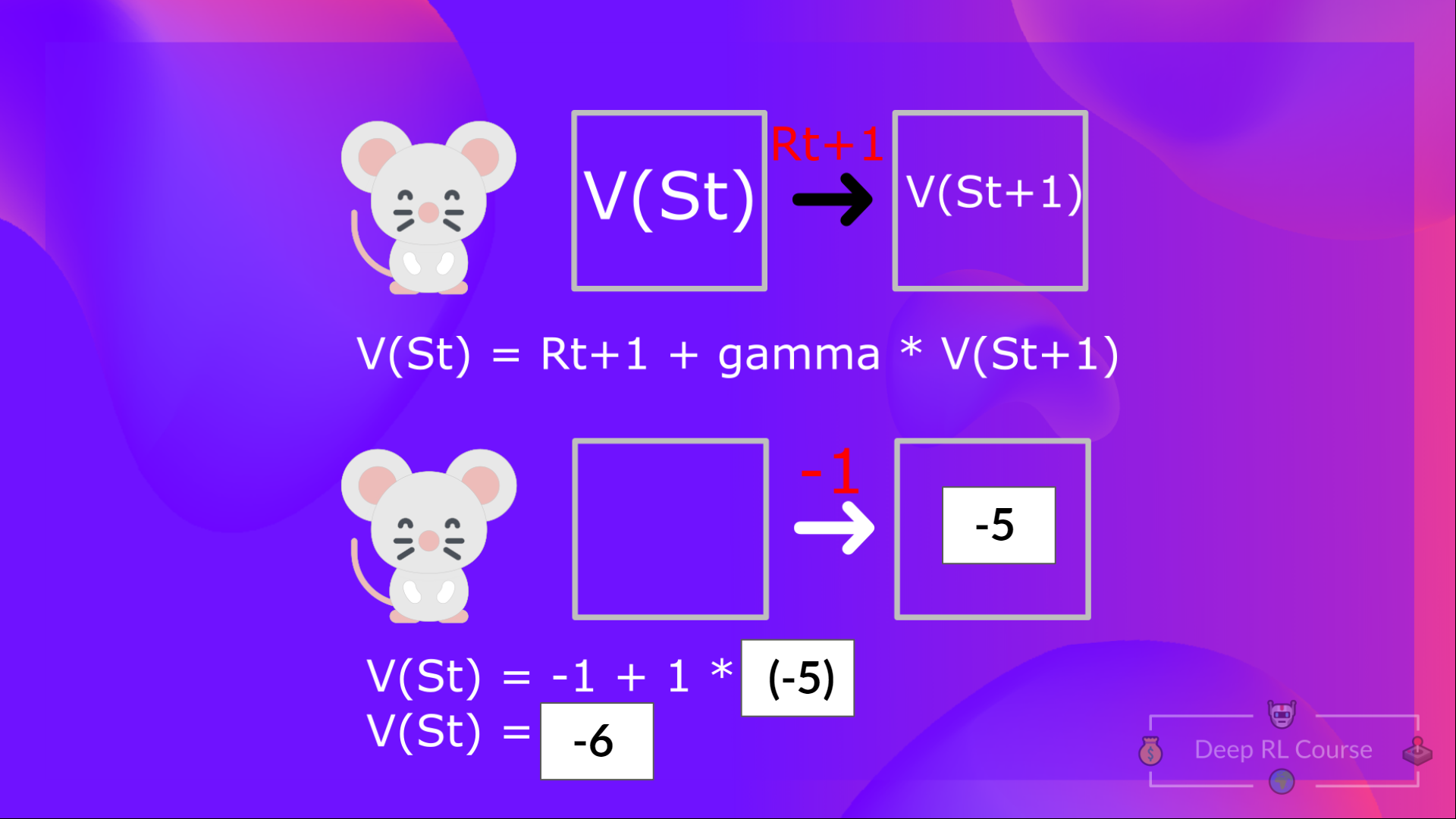
For simplification, here we do not discount, so gamma = 1.

• The worth of $V(S_{t+1})V(S\_\{t+1\})$
• And so forth.

To recap, the concept of the Bellman equation is that as a substitute of calculating each value because the sum of the expected return, which is an extended process. That is equivalent to the sum of immediate reward + the discounted value of the state that follows.

Monte Carlo vs Temporal Difference Learning

The final thing we’d like to discuss before diving into Q-Learning is the 2 ways of learning.

Keep in mind that an RL agent learns by interacting with its environment. The thought is that using the experience taken, given the reward it gets, will update its value or policy.

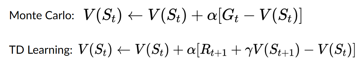
Monte Carlo and Temporal Difference Learning are two different strategies on the right way to train our worth function or our policy function. Each of them use experience to unravel the RL problem.

On one hand, Monte Carlo uses a complete episode of experience before learning. Then again, Temporal Difference uses only a step ( $S_t,A_t,R_{t+1},S_{t+1}S\_t,\; A\_t,\; R\_\{t+1\},\; S\_\{t+1\}$

We’ll explain each of them using a value-based method example.

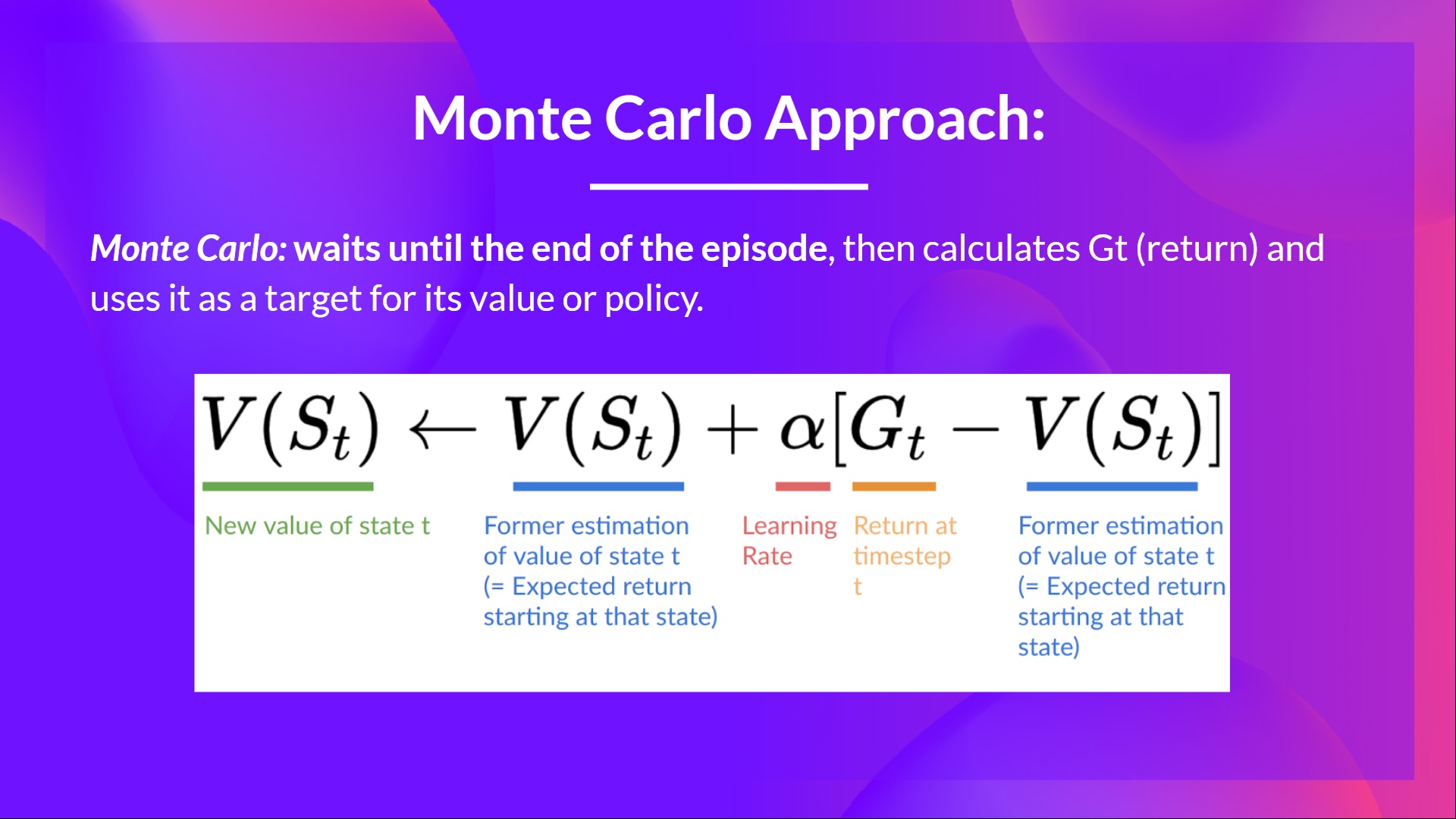
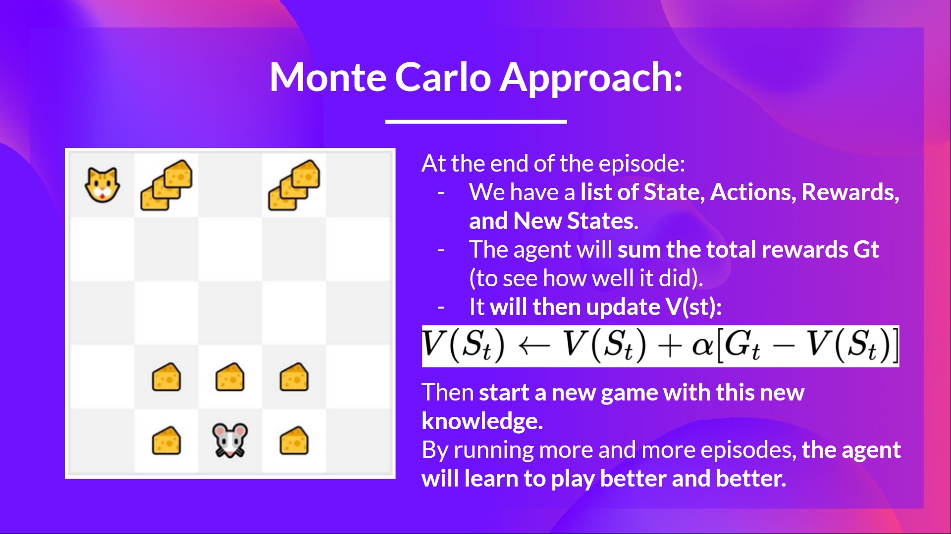
Monte Carlo: learning at the tip of the episode

Monte Carlo waits until the tip of the episode, calculates $G_{t}G\_t$

So it requires a complete entire episode of interaction before updating our worth function.

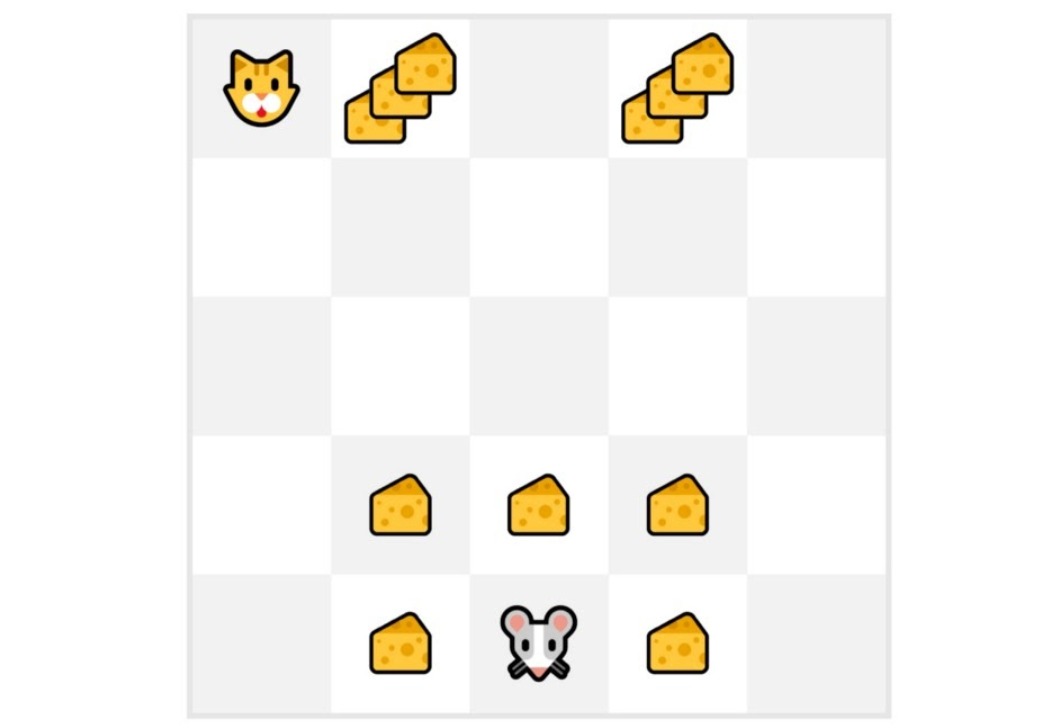
If we take an example:

• We at all times start the episode at the identical place to begin.

• The agent takes actions using the policy. As an illustration, using an Epsilon Greedy Strategy, a policy that alternates between exploration (random actions) and exploitation.

• We get the reward and the subsequent state.

• We terminate the episode if the cat eats the mouse or if the mouse moves > 10 steps.

• At the tip of the episode, we have now an inventory of State, Actions, Rewards, and Next States

• The agent will sum the entire rewards $G_{t}G\_t$ (to see how well it did).

• It should then update $V(s_t)V(s\_t)$

• Then start a brand new game with this recent knowledge

By running increasingly more episodes, the agent will learn to play higher and higher.

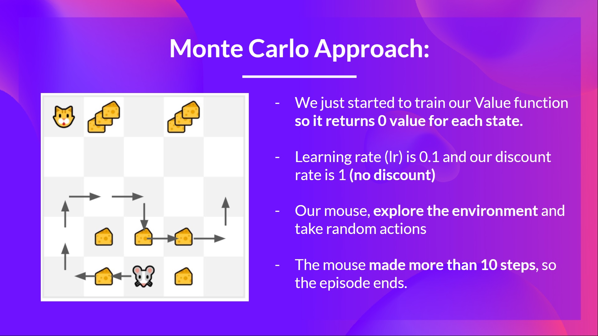
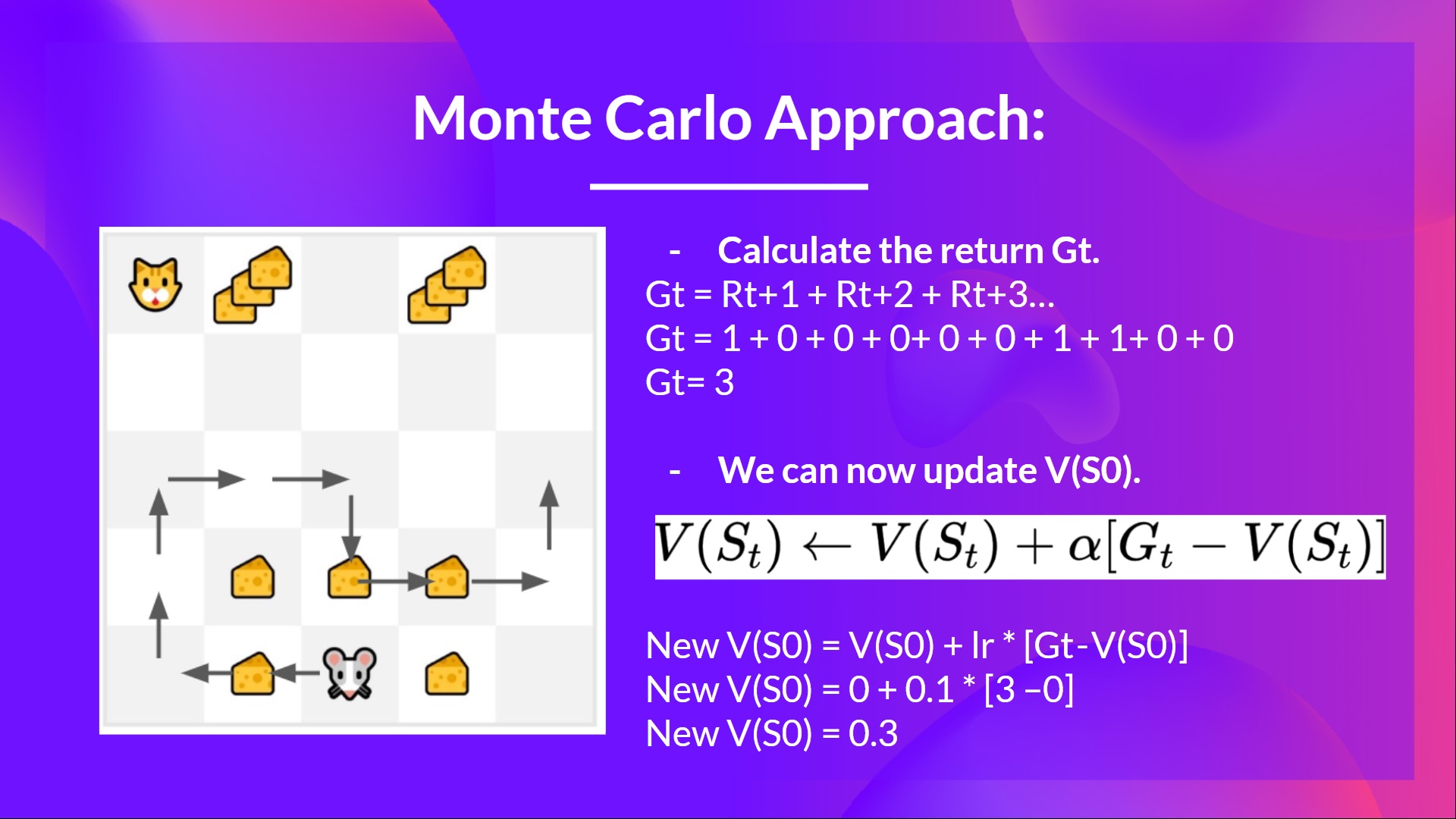
As an illustration, if we train a state-value function using Monte Carlo:

• We just began to train our Value function, so it returns 0 value for every state
• Our learning rate (lr) is 0.1 and our discount rate is 1 (= no discount)
• Our mouse explores the environment and takes random actions

• The mouse made greater than 10 steps, so the episode ends .

• We’ve got an inventory of state, motion, rewards, next_state, we’d like to calculate the return $GtG\{t\}$
• $G_t=R_{t+1}+R_{t+2}+R_{t+3}\mathrm{.}\mathrm{.}\mathrm{.}G\_t\; =\; R\_\{t+1\}\; +\; R\_\{t+2\}\; +\; R\_\{t+3\}\; \dots$
• $G_t=R_{t+1}+R_{t+2}+R_{t+3}\dots G\_t\; =\; R\_\{t+1\}\; +\; R\_\{t+2\}\; +\; R\_\{t+3\}\dots$
• $G_t=1+0+0+0+0+0+1+1+0+0G\_t\; =\; 1\; +\; 0\; +\; 0\; +\; 0+\; 0\; +\; 0\; +\; 1\; +\; 1\; +\; 0\; +\; 0$
• $G_t=3G\_t=\; 3$
• We will now update $V(S_0)V(S\_0)$

• Recent $V(S_0)=V(S_0)+lr\ast [G_t\text{—}V(S_0)]V(S\_0)\; =\; V(S\_0)\; +\; lr\; *\; [G\_t\; —\; V(S\_0)]$
• Recent $V(S_0)=0+0.1\ast [3\text{–}0]V(S\_0)\; =\; 0\; +\; 0.1\; *\; [3\; –\; 0]$
• Recent $V(S_0)=0.3V(S\_0)\; =\; 0.3$

Temporal Difference Learning: learning at each step

• Temporal difference, alternatively, waits for under one interaction (one step) $S_{t+1}S\_\{t+1\}$
• to form a TD goal and update $V(S_t)V(S\_t)$

The thought with TD is to update the $V(S_t)V(S\_t)$

But because we didn’t play during a complete episode, we do not have $G_{t}G\_t$

This is known as bootstrapping. It’s called this because TD bases its update part on an existing estimate $V(S_{t+1})V(S\_\{t+1\})$

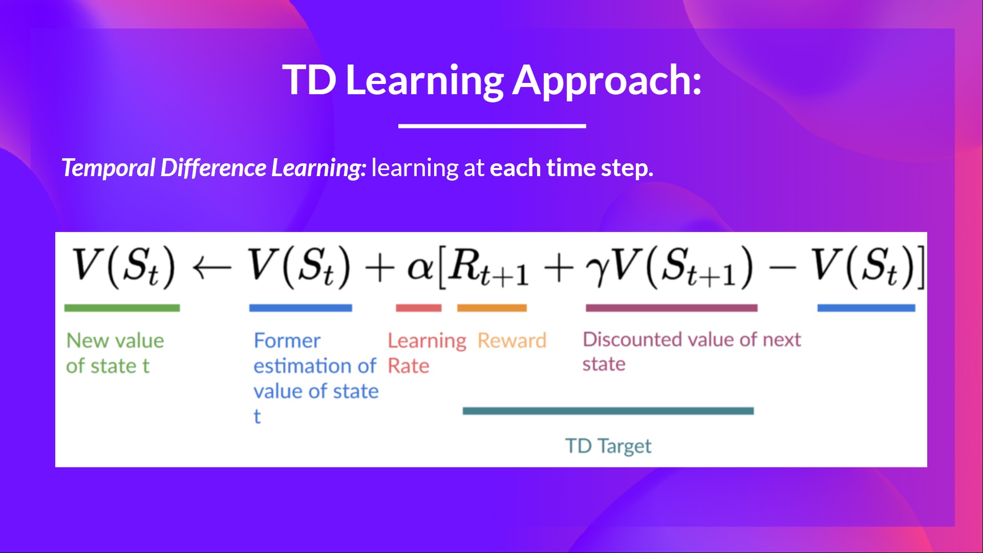
This method is known as TD(0) or one-step TD (update the worth function after any individual step).

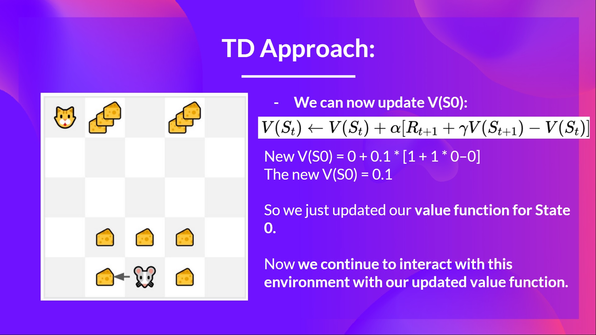
If we take the identical example,

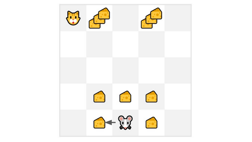
• We just began to train our Value function, so it returns 0 value for every state.
• Our learning rate (lr) is 0.1, and our discount rate is 1 (no discount).
• Our mouse explore the environment and take a random motion: going to the left
• It gets a reward $R_{t+1}=1R\_\{t+1\}\; =\; 1$

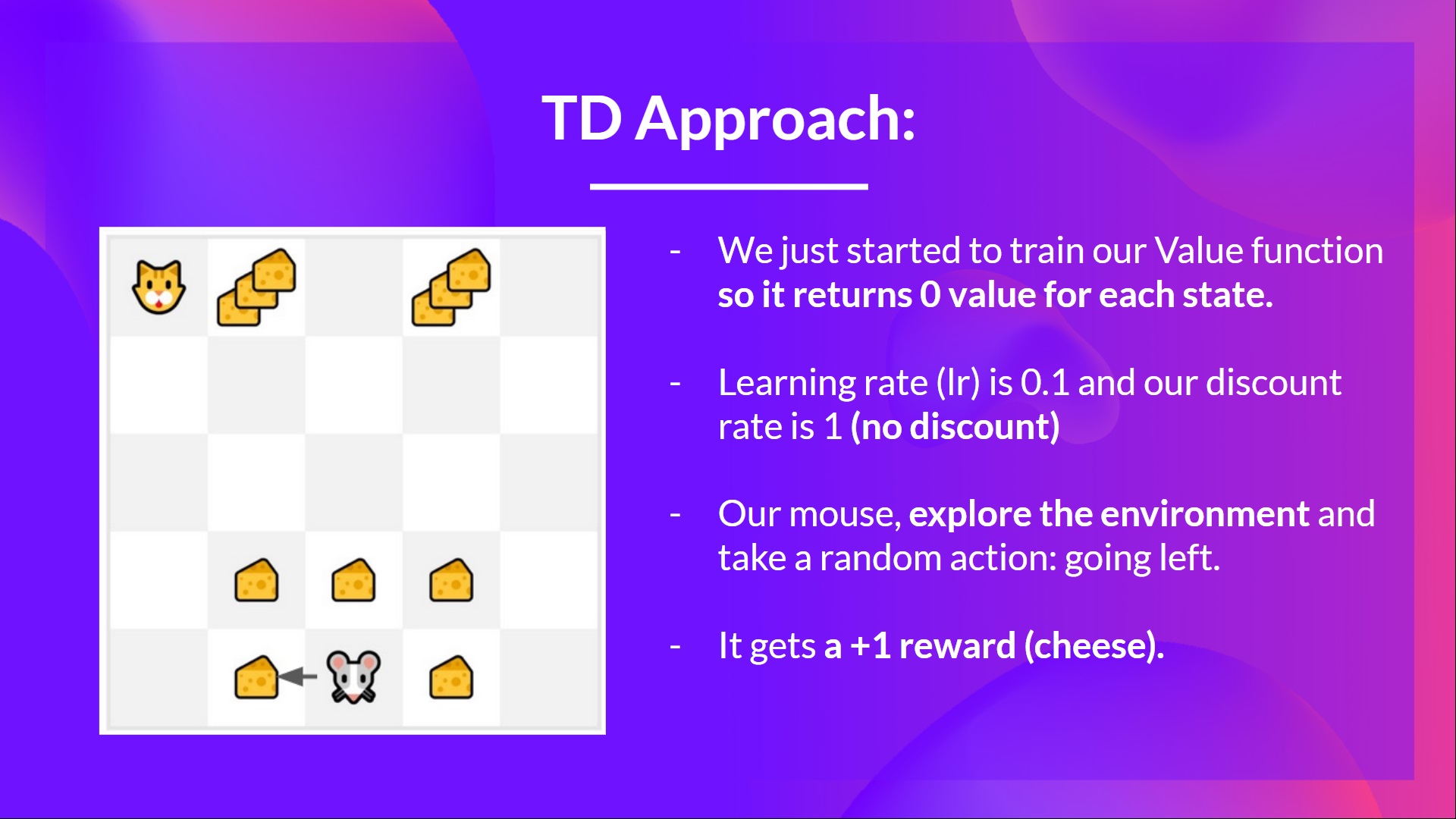
We will now update $V(S_0)V(S\_0)$

Recent $V(S_0)=V(S_0)+lr\ast [R_1+gamma\ast V(S_1)-V(S_0)]V(S\_0)\; =\; V(S\_0)\; +\; lr\; *\; [R\_1\; +\; gamma\; *\; V(S\_1)\; –\; V(S\_0)]$

Recent $V(S_0)=0+0.1\ast [1+1\ast 0\text{–}0]V(S\_0)\; =\; 0\; +\; 0.1\; *\; [1\; +\; 1\; *\; 0–0]$

Recent $V(S_0)=0.1V(S\_0)\; =\; 0.1$

So we just updated our worth function for State 0.

Now we proceed to interact with this environment with our updated value function.

If we summarize:

• With Monte Carlo, we update the worth function from a whole episode, and so we use the actual accurate discounted return of this episode.
• With TD learning, we update the worth function from a step, so we replace $G_{t}G\_t$

So now, before diving on Q-Learning, let’s summarise what we just learned:

We’ve got two kinds of value-based functions:

• State-Value function: outputs the expected return if the agent starts at a given state and acts accordingly to the policy eternally after.
• Motion-Value function: outputs the expected return if the agent starts in a given state, takes a given motion at that state after which acts accordingly to the policy eternally after.
• In value-based methods, we define the policy by hand because we do not train it, we train a price function. The thought is that if we have now an optimal value function, we can have an optimal policy.

There are two kinds of methods to learn a policy for a price function:

• With the Monte Carlo method, we update the worth function from a whole episode, and so we use the actual accurate discounted return of this episode.
• With the TD Learning method, we update the worth function from a step, so we replace Gt that we do not have with an estimated return called TD goal.

In order that’s all for today. Congrats on ending this primary a part of the chapter! There was plenty of information.

That’s normal when you still feel confused with all these elements. This was the identical for me and for all individuals who studied RL.

Take time to actually grasp the fabric before continuing.

And since the most effective strategy to learn and avoid the illusion of competence is to check yourself. We wrote a quiz to provide help to find where you’ll want to reinforce your study.
Check your knowledge here 👉 https://github.com/huggingface/deep-rl-class/blob/most important/unit2/quiz1.md

Within the second part , we’ll study our first RL algorithm: Q-Learning, and implement our first RL Agent in two environments:

1. Frozen-Lake-v1 (non-slippery version): where our agent might want to go from the starting state (S) to the goal state (G) by walking only on frozen tiles (F) and avoiding holes (H).
2. An autonomous taxi will need to learn to navigate a city to transport its passengers from point A to point B.

And remember to share with your mates who need to learn 🤗 !

Finally, we wish to enhance and update the course iteratively along with your feedback. If you may have some, please fill this way 👉 https://forms.gle/3HgA7bEHwAmmLfwh9

Continue to learn, stay awesome,