


⚠️ A latest updated version of this text is offered here 👉 https://huggingface.co/deep-rl-course/unit1/introduction
This text is an element of the Deep Reinforcement Learning Class. A free course from beginner to expert. Check the syllabus here.
⚠️ A latest updated version of this text is offered here 👉 https://huggingface.co/deep-rl-course/unit1/introduction
This text is an element of the Deep Reinforcement Learning Class. A free course from beginner to expert. Check the syllabus here.
Within the last unit, we learned our first reinforcement learning algorithm: Q-Learning, implemented it from scratch, and trained it in two environments, FrozenLake-v1 ☃️ and Taxi-v3 🚕.
We got excellent results with this straightforward algorithm. But these environments were relatively easy since the State Space was discrete and small (14 different states for FrozenLake-v1 and 500 for Taxi-v3).
But as we’ll see, producing and updating a Q-table can change into ineffective in large state space environments.
So today, we’ll study our first Deep Reinforcement Learning agent: Deep Q-Learning. As an alternative of using a Q-table, Deep Q-Learning uses a Neural Network that takes a state and approximates Q-values for every motion based on that state.
And we’ll train it to play Space Invaders and other Atari environments using RL-Zoo, a training framework for RL using Stable-Baselines that gives scripts for training, evaluating agents, tuning hyperparameters, plotting results, and recording videos.
So let’s start! 🚀
To have the opportunity to grasp this unit, you’ll want to understand Q-Learning first.
From Q-Learning to Deep Q-Learning
We learned that Q-Learning is an algorithm we use to coach our Q-Function, an action-value function that determines the worth of being at a selected state and taking a selected motion at that state.
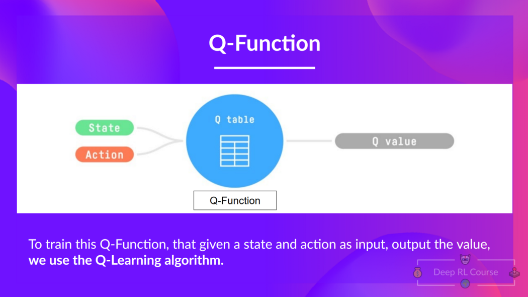
The Q comes from “the Quality” of that motion at that state.
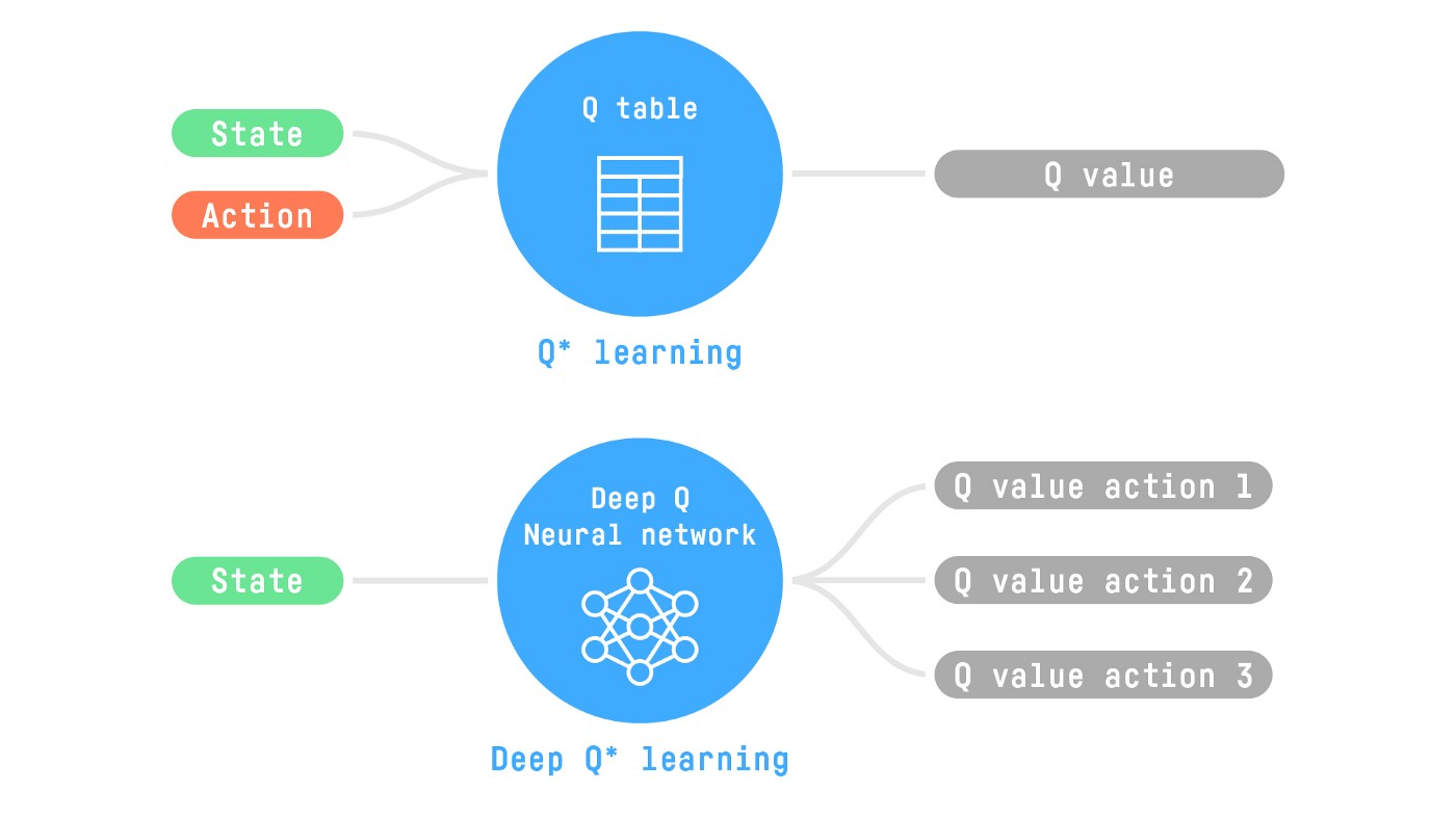
Internally, our Q-function has a Q-table, a table where each cell corresponds to a state-action pair value. Consider this Q-table as the memory or cheat sheet of our Q-function.
The issue is that Q-Learning is a tabular method. Aka, an issue during which the state and actions spaces are sufficiently small to approximate value functions to be represented as arrays and tables. And that is not scalable.
Q-Learning was working well with small state space environments like:
- FrozenLake, we had 14 states.
- Taxi-v3, we had 500 states.
But consider what we will do today: we’ll train an agent to learn to play Space Invaders using the frames as input.
As Nikita Melkozerov mentioned, Atari environments have an statement space with a shape of (210, 160, 3), containing values starting from 0 to 255 so that provides us 256^(210x160x3) = 256^100800 (for comparison, we have now roughly 10^80 atoms within the observable universe).
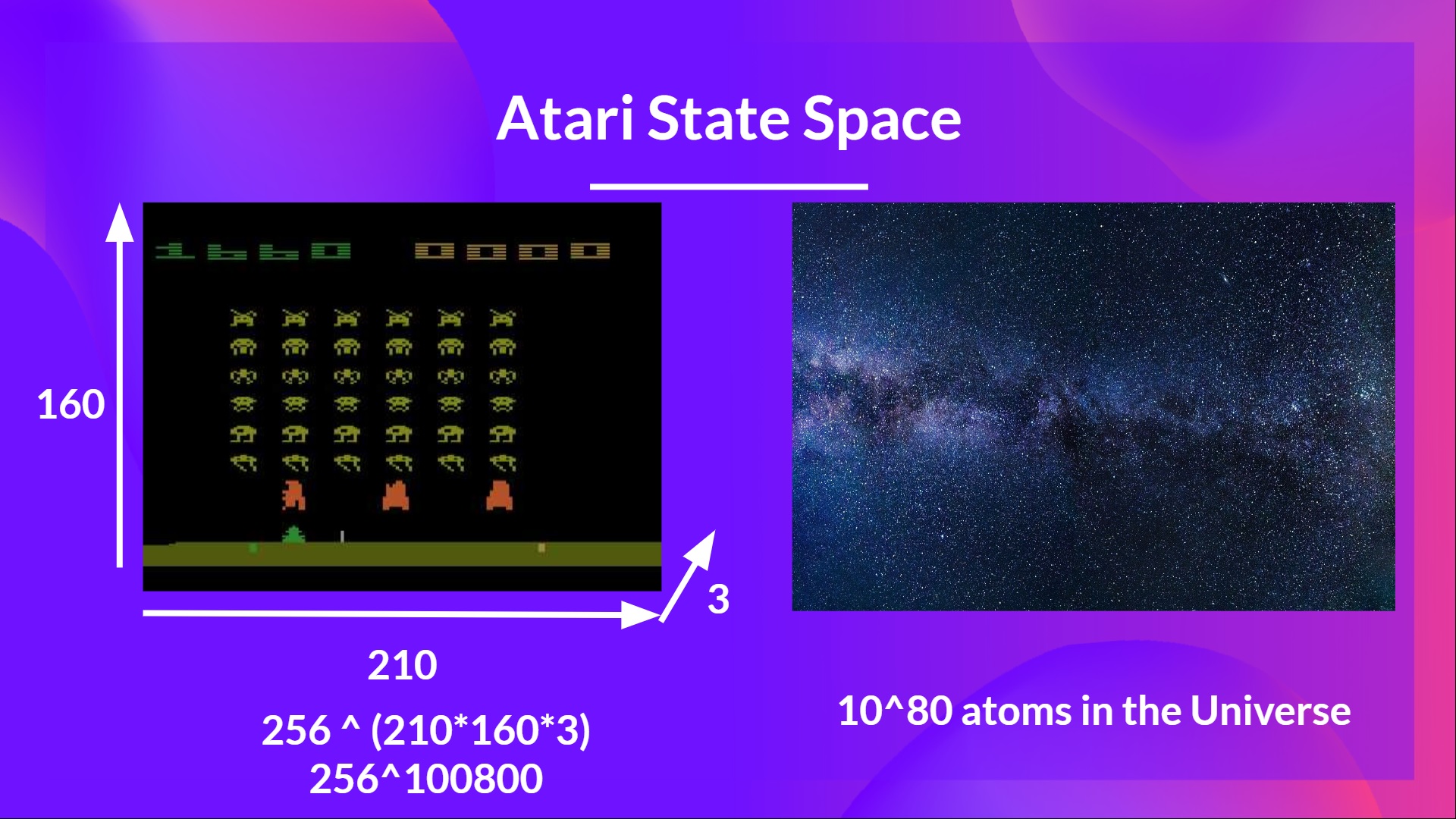
Subsequently, the state space is gigantic; hence creating and updating a Q-table for that environment wouldn’t be efficient. On this case, the most effective idea is to approximate the Q-values as a substitute of a Q-table using a parametrized Q-function .
This neural network will approximate, given a state, different Q-values for every possible motion at that state. And that is exactly what Deep Q-Learning does.
Now that we understand Deep Q-Learning, let’s dive deeper into the Deep Q-Network.
The Deep Q-Network (DQN)
That is the architecture of our Deep Q-Learning network:
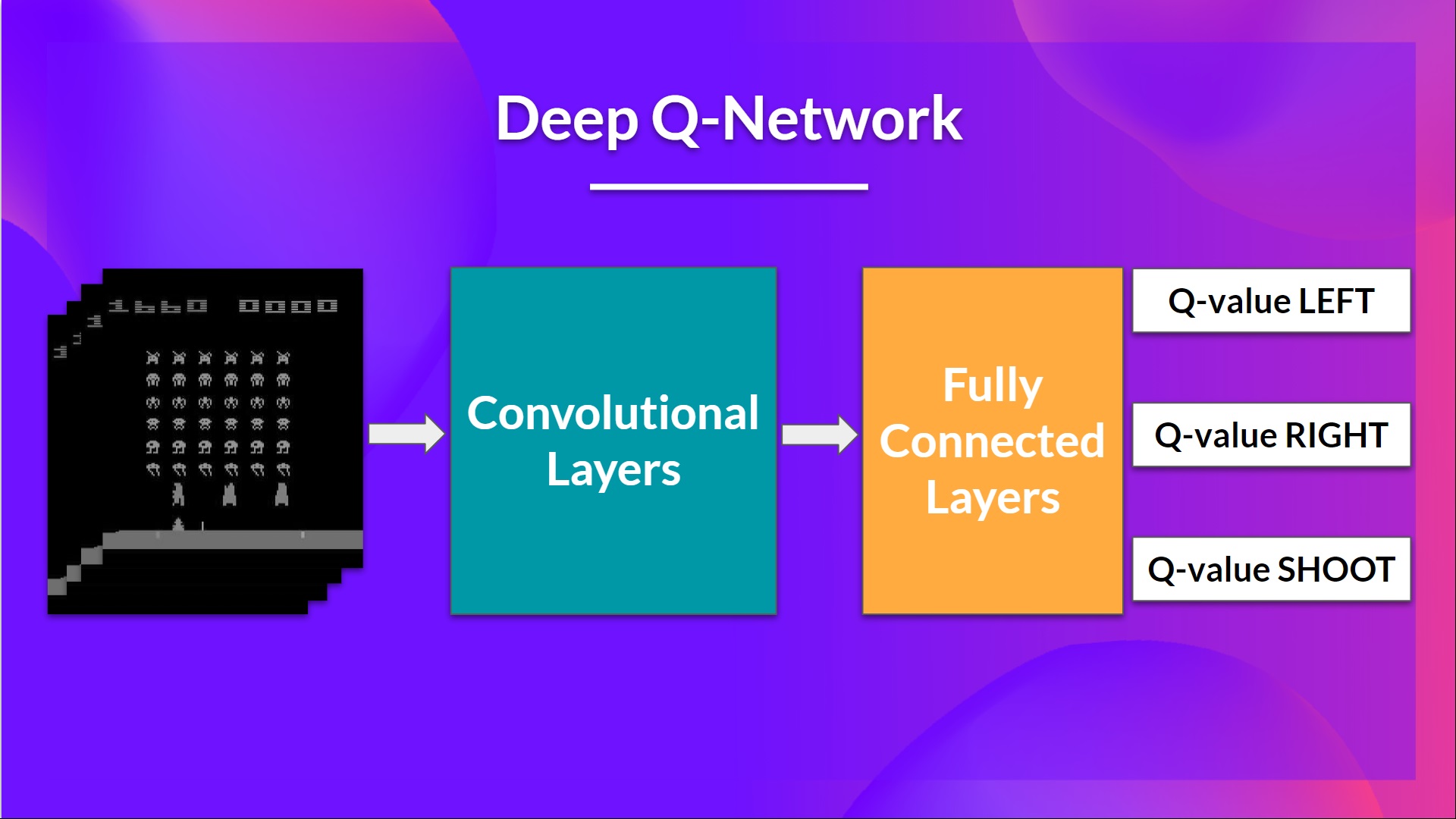
As input, we take a stack of 4 frames passed through the network as a state and output a vector of Q-values for every possible motion at that state. Then, like with Q-Learning, we just need to make use of our epsilon-greedy policy to pick which motion to take.
When the Neural Network is initialized, the Q-value estimation is terrible. But during training, our Deep Q-Network agent will associate a situation with appropriate motion and learn to play the sport well.
Preprocessing the input and temporal limitation
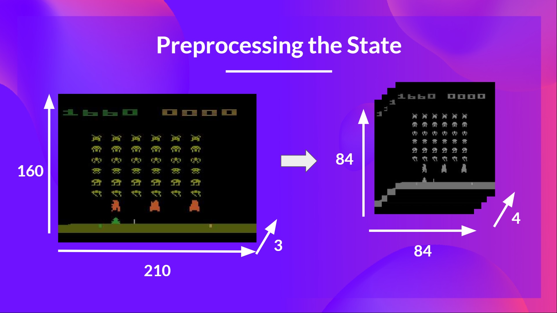
We mentioned that we preprocess the input. It’s an important step since we wish to cut back the complexity of our state to cut back the computation time needed for training.
So what we do is reduce the state space to 84×84 and grayscale it (for the reason that colours in Atari environments don’t add essential information).
That is an important saving since we reduce our three color channels (RGB) to 1.
We also can crop an element of the screen in some games if it doesn’t contain essential information.
Then we stack 4 frames together.
Why will we stack 4 frames together?
We stack frames together since it helps us handle the issue of temporal limitation. Let’s take an example with the sport of Pong. While you see this frame:
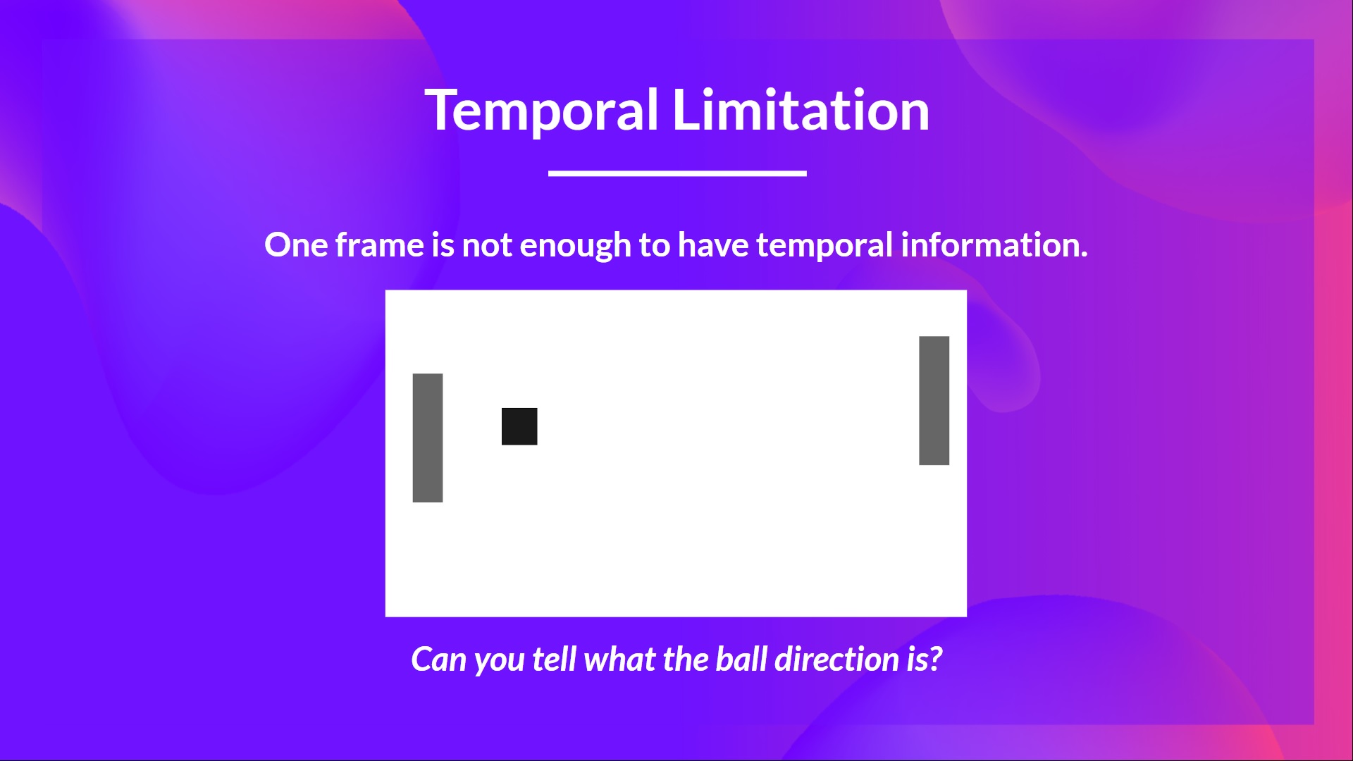
Are you able to tell me where the ball goes?
No, because one frame just isn’t enough to have a way of motion! But what if I add three more frames? Here you possibly can see that the ball goes to the correct.
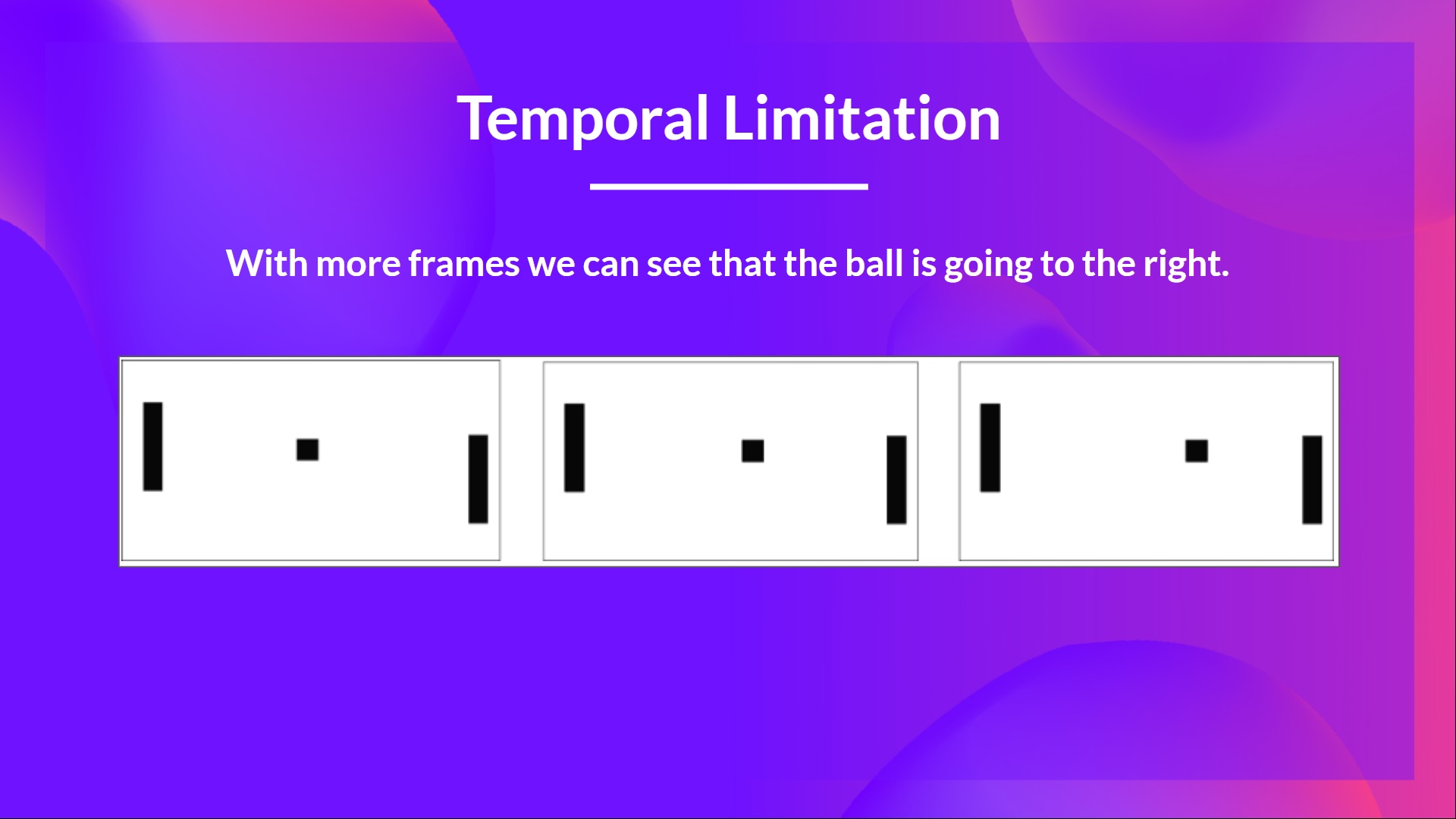
That’s why, to capture temporal information, we stack 4 frames together.
Then, the stacked frames are processed by three convolutional layers. These layers allow us to capture and exploit spatial relationships in images. But in addition, because frames are stacked together, you possibly can exploit some spatial properties across those frames.
Finally, we have now a few fully connected layers that output a Q-value for every possible motion at that state.
So, we see that Deep Q-Learning is using a neural network to approximate, given a state, different Q-values for every possible motion at that state. Let’s now study the Deep Q-Learning algorithm.
The Deep Q-Learning Algorithm
We learned that Deep Q-Learning uses a deep neural network to approximate different Q-values for every possible motion at a state (value-function estimation).
The difference is that, through the training phase, as a substitute of updating the Q-value of a state-action pair directly as we have now done with Q-Learning:
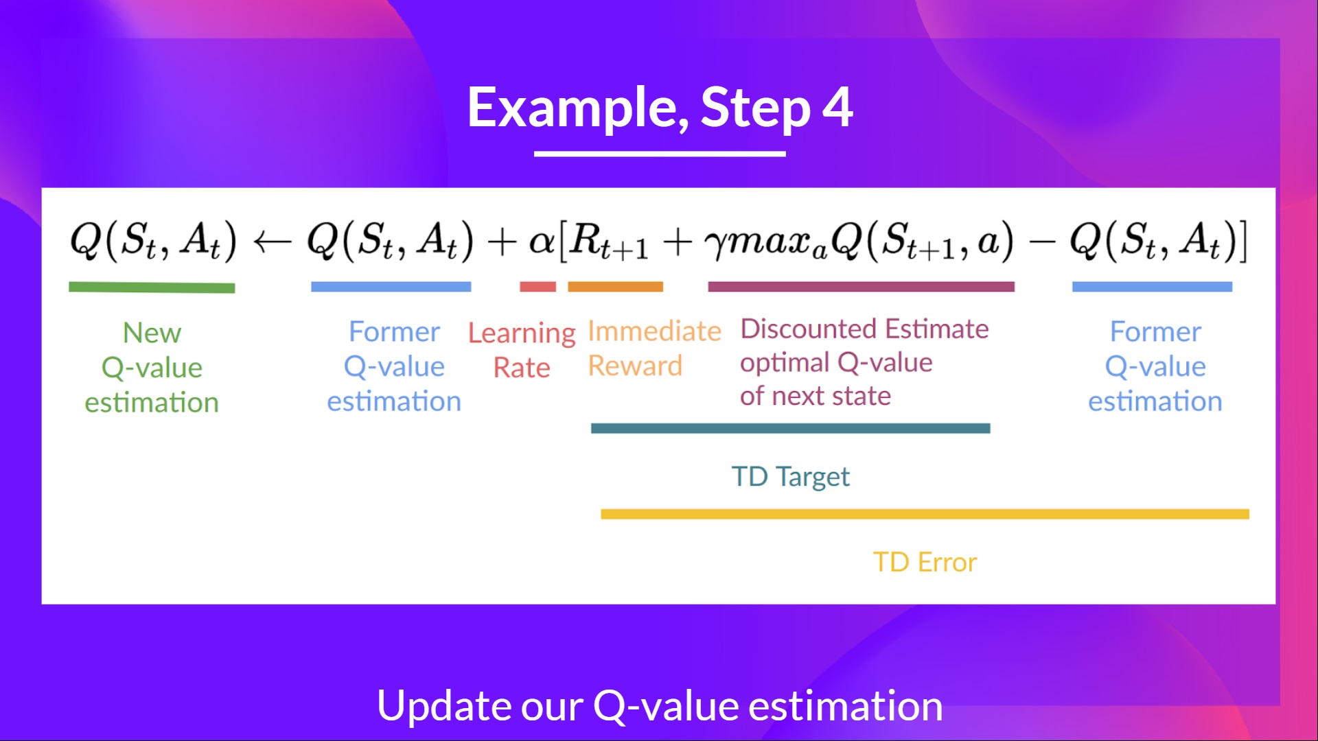
In Deep Q-Learning, we create a Loss function between our Q-value prediction and the Q-target and use Gradient Descent to update the weights of our Deep Q-Network to approximate our Q-values higher.
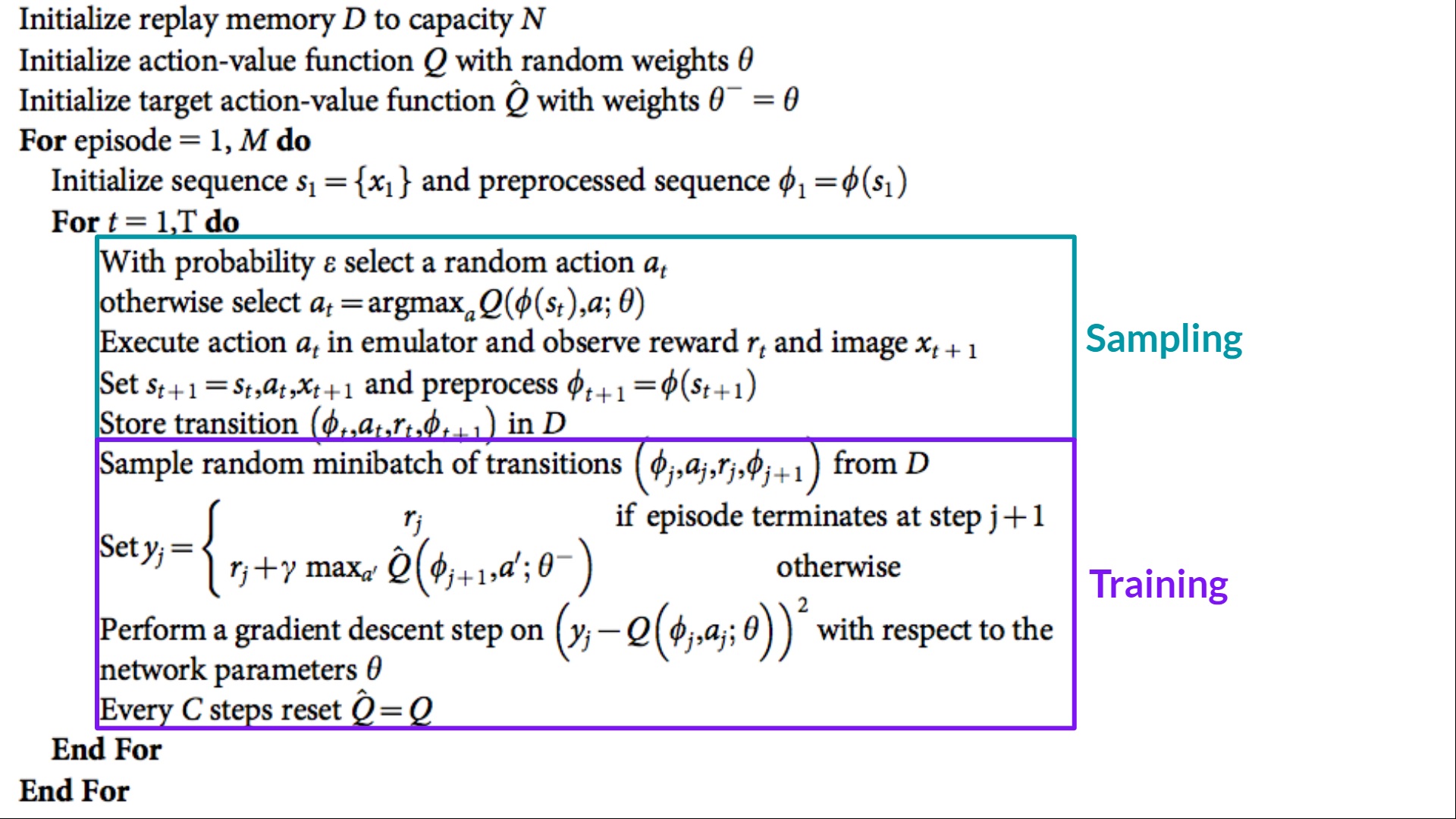
The Deep Q-Learning training algorithm has two phases:
- Sampling: we perform actions and store the observed experiences tuples in a replay memory.
- Training: Select the small batch of tuple randomly and learn from it using a gradient descent update step.
But, this just isn’t the one change compared with Q-Learning. Deep Q-Learning training might suffer from instability, mainly because of mixing a non-linear Q-value function (Neural Network) and bootstrapping (once we update targets with existing estimates and never an actual complete return).
To assist us stabilize the training, we implement three different solutions:
- Experience Replay, to make more efficient use of experiences.
- Fixed Q-Goal to stabilize the training.
- Double Deep Q-Learning, to handle the issue of the overestimation of Q-values.
Experience Replay to make more efficient use of experiences
Why will we create a replay memory?
Experience Replay in Deep Q-Learning has two functions:
- Make more efficient use of the experiences through the training.
- Experience replay helps us make more efficient use of the experiences through the training. Often, in online reinforcement learning, we interact within the environment, get experiences (state, motion, reward, and next state), learn from them (update the neural network) and discard them.
- But with experience replay, we create a replay buffer that saves experience samples that we will reuse through the training.

⇒ This permits us to learn from individual experiences multiple times.
- Avoid forgetting previous experiences and reduce the correlation between experiences.
- The issue we get if we give sequential samples of experiences to our neural network is that it tends to forget the previous experiences because it overwrites latest experiences. For example, if we’re in the primary level after which the second, which is different, our agent can forget tips on how to behave and play in the primary level.
The answer is to create a Replay Buffer that stores experience tuples while interacting with the environment after which sample a small batch of tuples. This prevents the network from only learning about what it has immediately done.
Experience replay also has other advantages. By randomly sampling the experiences, we remove correlation within the statement sequences and avoid motion values from oscillating or diverging catastrophically.
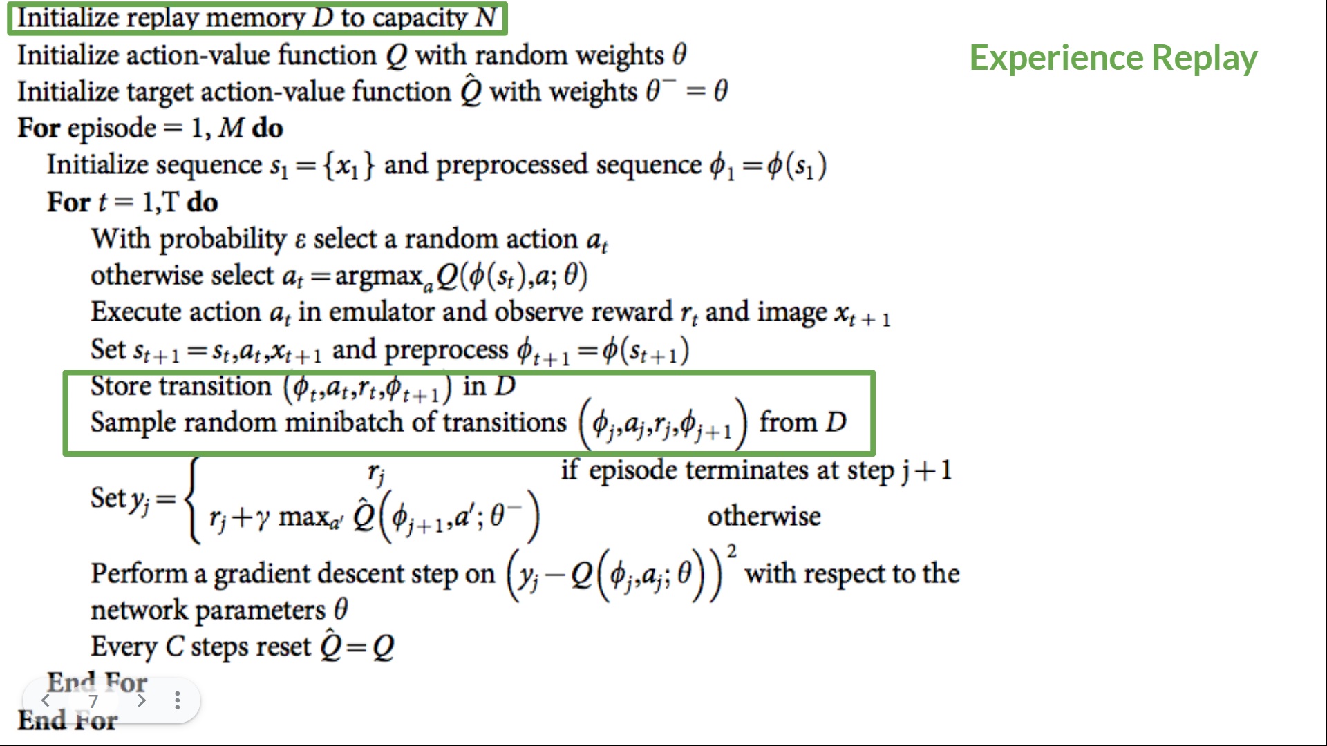
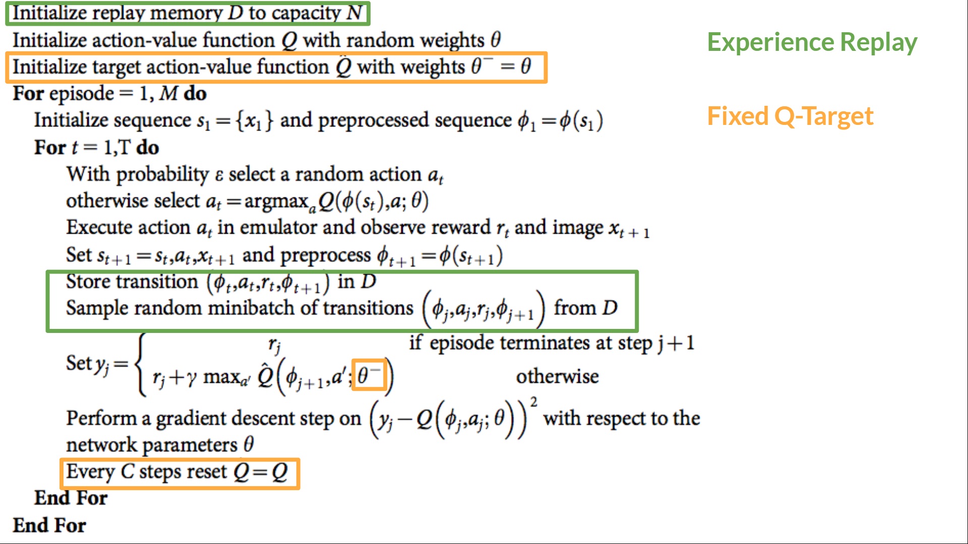
Within the Deep Q-Learning pseudocode, we see that we initialize a replay memory buffer D from capability N (N is an hyperparameter you can define). We then store experiences within the memory and sample a minibatch of experiences to feed the Deep Q-Network through the training phase.
Fixed Q-Goal to stabilize the training
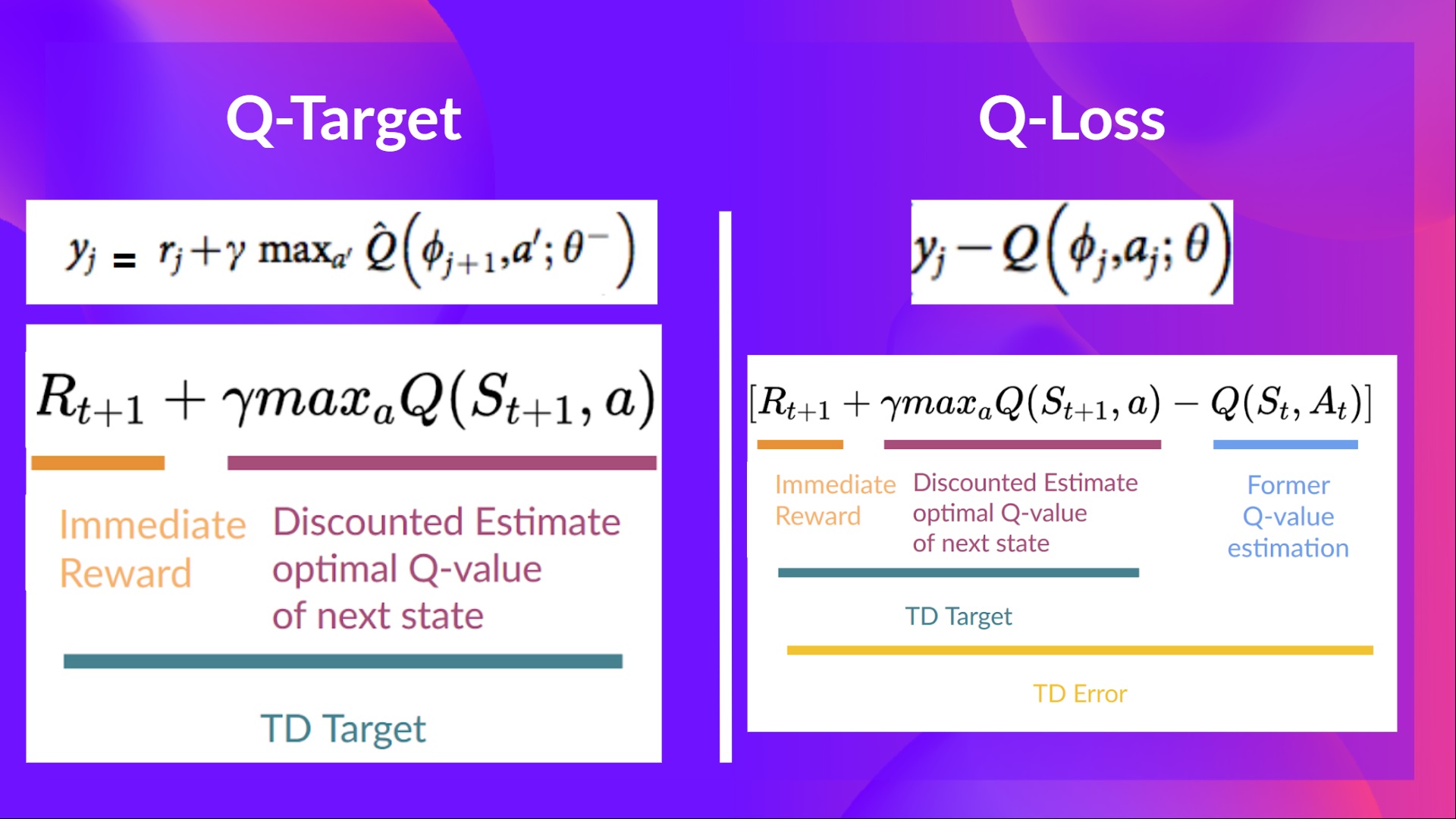
When we wish to calculate the TD error (aka the loss), we calculate the difference between the TD goal (Q-Goal) and the present Q-value (estimation of Q).
But we don’t have any idea of the actual TD goal. We’d like to estimate it. Using the Bellman equation, we saw that the TD goal is just the reward of taking that motion at that state plus the discounted highest Q value for the following state.
Nevertheless, the issue is that we’re using the identical parameters (weights) for estimating the TD goal and the Q value. Consequently, there’s a big correlation between the TD goal and the parameters we’re changing.
Subsequently, it implies that at every step of coaching, our Q values shift but in addition the goal value shifts. So, we’re getting closer to our goal, however the goal can be moving. It’s like chasing a moving goal! This led to a big oscillation in training.
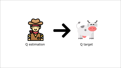
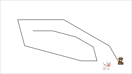
It’s like if you happen to were a cowboy (the Q estimation) and you must catch the cow (the Q-target), you should catch up with (reduce the error).
At every time step, you’re attempting to approach the cow, which also moves at every time step (because you utilize the identical parameters).
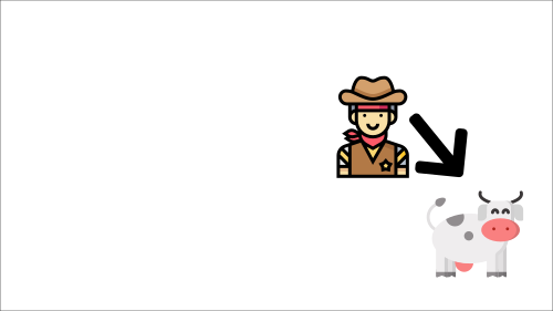
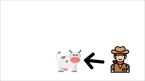
This results in a bizarre path of chasing (a big oscillation in training).
As an alternative, what we see within the pseudo-code is that we:
- Use a separate network with a set parameter for estimating the TD Goal
- Copy the parameters from our Deep Q-Network at every C step to update the goal network.
Double DQN
Double DQNs, or Double Learning, were introduced by Hado van Hasselt. This method handles the issue of the overestimation of Q-values.
To know this problem, remember how we calculate the TD Goal:
We face an easy problem by calculating the TD goal: how are we sure that the most effective motion for the following state is the motion with the very best Q-value?
We all know that the accuracy of Q values depends upon what motion we tried and what neighboring states we explored.
Consequently, we don’t have enough details about the most effective motion to take firstly of the training. Subsequently, taking the utmost Q value (which is noisy) as the most effective motion to take can result in false positives. If non-optimal actions are repeatedly given the next Q value than the optimal best motion, the training might be complicated.
The answer is: once we compute the Q goal, we use two networks to decouple the motion selection from the goal Q value generation. We:
- Use our DQN network to pick the most effective motion to take for the following state (the motion with the very best Q value).
- Use our Goal network to calculate the goal Q value of taking that motion at the following state.
Subsequently, Double DQN helps us reduce the overestimation of q values and, as a consequence, helps us train faster and have more stable learning.
Since these three improvements in Deep Q-Learning, many have been added corresponding to Prioritized Experience Replay, Dueling Deep Q-Learning. They’re out of the scope of this course but if you happen to’re interested, check the links we put within the reading list. 👉 https://github.com/huggingface/deep-rl-class/blob/fundamental/unit3/README.md
Now that you have studied the speculation behind Deep Q-Learning, you’re able to train your Deep Q-Learning agent to play Atari Games. We’ll start with Space Invaders, but you will have the opportunity to make use of any Atari game you wish 🔥
We’re using the RL-Baselines-3 Zoo integration, a vanilla version of Deep Q-Learning with no extensions corresponding to Double-DQN, Dueling-DQN, and Prioritized Experience Replay.
Start the tutorial here 👉 https://colab.research.google.com/github/huggingface/deep-rl-class/blob/fundamental/unit3/unit3.ipynb
The leaderboard to match your results along with your classmates 🏆 👉 https://huggingface.co/spaces/chrisjay/Deep-Reinforcement-Learning-Leaderboard
Congrats on ending this chapter! There was a number of information. And congrats on ending the tutorial. You’ve just trained your first Deep Q-Learning agent and shared it on the Hub 🥳.
That’s normal if you happen to still feel confused with all these elements. This was the identical for me and for all individuals who studied RL.
Take time to essentially grasp the fabric before continuing.
Don’t hesitate to coach your agent in other environments (Pong, Seaquest, QBert, Ms Pac Man). The best technique to learn is to try things on your personal!
We published additional readings within the syllabus if you must go deeper 👉 https://github.com/huggingface/deep-rl-class/blob/fundamental/unit3/README.md
In the following unit, we’re going to find out about Policy Gradients methods.
And do not forget to share with your folks who wish to learn 🤗 !
Finally, we wish to enhance and update the course iteratively along with your feedback. If you could have some, please fill this manner 👉 https://forms.gle/3HgA7bEHwAmmLfwh9