

⚠️ A latest updated version of this text is on the market here 👉 https://huggingface.co/deep-rl-course/unit1/introduction
This text is a component of the Deep Reinforcement Learning Class. A free course from beginner to expert. Check the syllabus here.
⚠️ A latest updated version of this text is on the market here 👉 https://huggingface.co/deep-rl-course/unit1/introduction
This text is a component of the Deep Reinforcement Learning Class. A free course from beginner to expert. Check the syllabus here.
Within the last unit, we learned about Deep Q-Learning. On this value-based Deep Reinforcement Learning algorithm, we used a deep neural network to approximate different Q-values for every possible motion at a state.
Indeed, because the starting of the course, we only studied value-based methods, where we estimate a price function as an intermediate step towards finding an optimal policy.
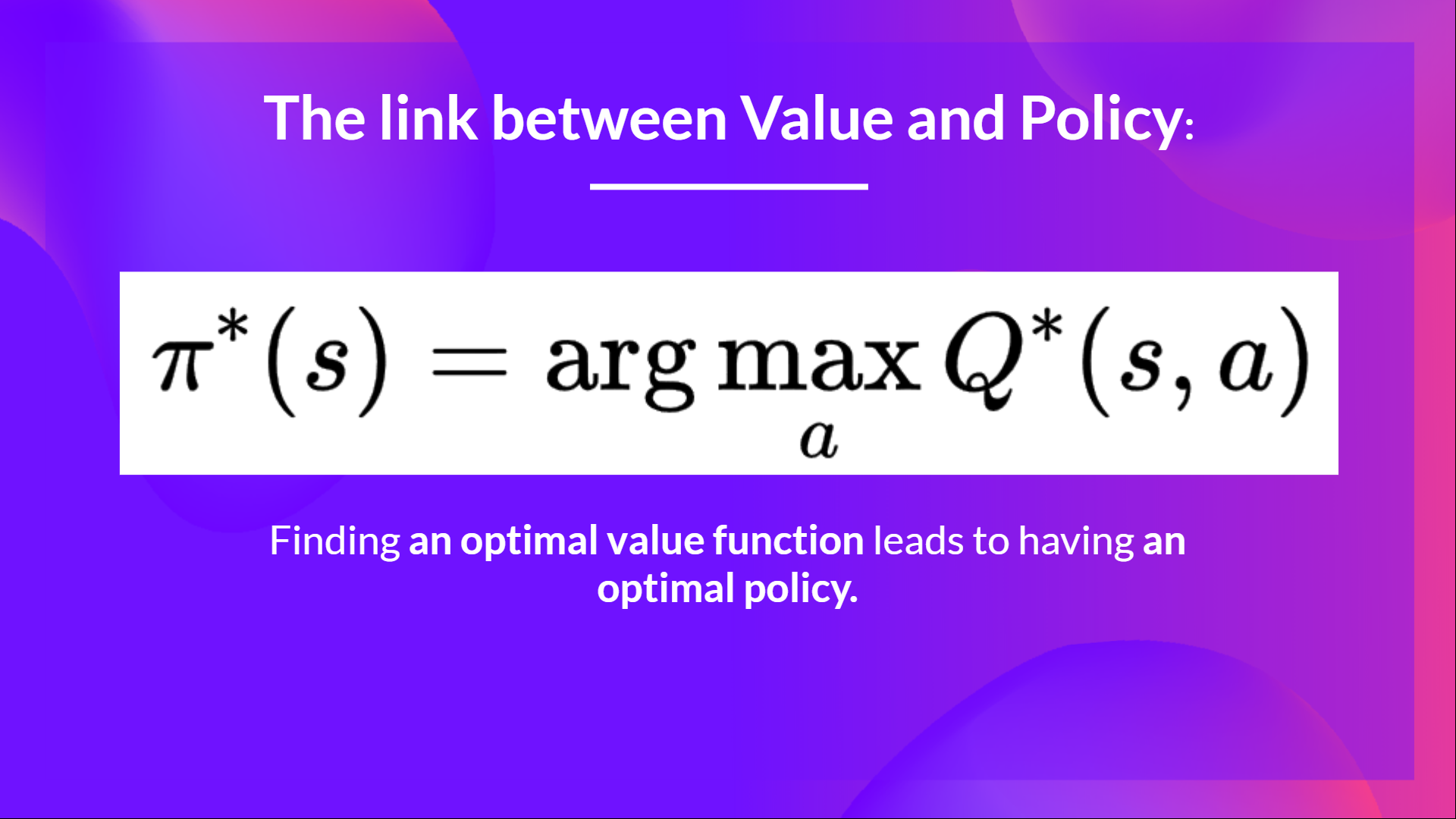
Because, in value-based, π exists only due to motion value estimates, since policy is only a function (as an example, greedy-policy) that may select the motion with the very best value given a state.
But, with policy-based methods, we wish to optimize the policy directly without having an intermediate step of learning a price function.
So today, we’ll study our first Policy-Based method: Reinforce. And we’ll implement it from scratch using PyTorch. Before testing its robustness using CartPole-v1, PixelCopter, and Pong.

Let’s start,
What are Policy-Gradient Methods?
Policy-Gradient is a subclass of Policy-Based Methods, a category of algorithms that goals to optimize the policy directly without using a price function using different techniques. The difference with Policy-Based Methods is that Policy-Gradient methods are a series of algorithms that aim to optimize the policy directly by estimating the weights of the optimal policy using Gradient Ascent.
An Overview of Policy Gradients
Why can we optimize the policy directly by estimating the weights of an optimal policy using Gradient Ascent in Policy Gradients Methods?
Keep in mind that reinforcement learning goals to search out an optimal behavior strategy (policy) to maximise its expected cumulative reward.
We also must keep in mind that a policy is a function that given a state, outputs, a distribution over actions (in our case using a stochastic policy).
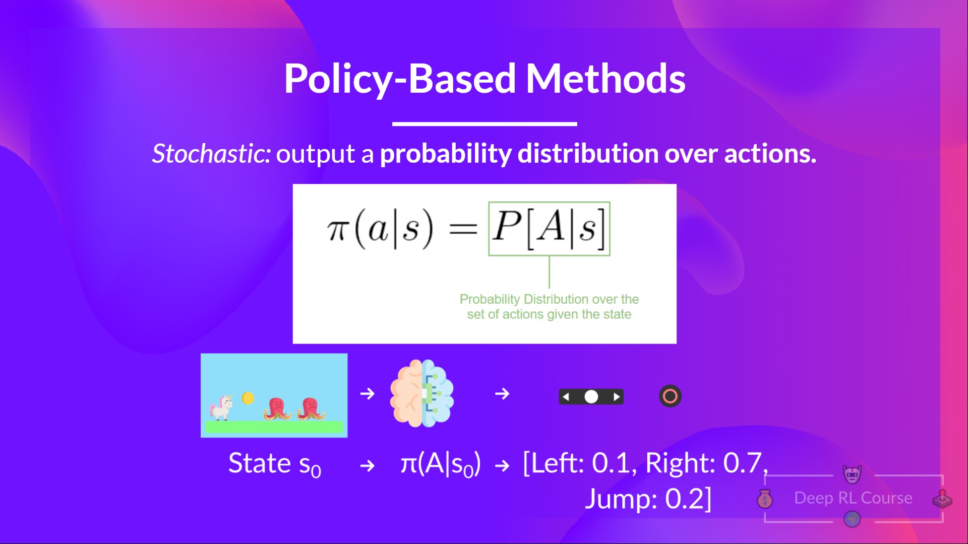
Our goal with Policy-Gradients is to manage the probability distribution of actions by tuning the policy such that good actions (that maximize the return) are sampled more ceaselessly in the longer term.
Let’s take a straightforward example:
-
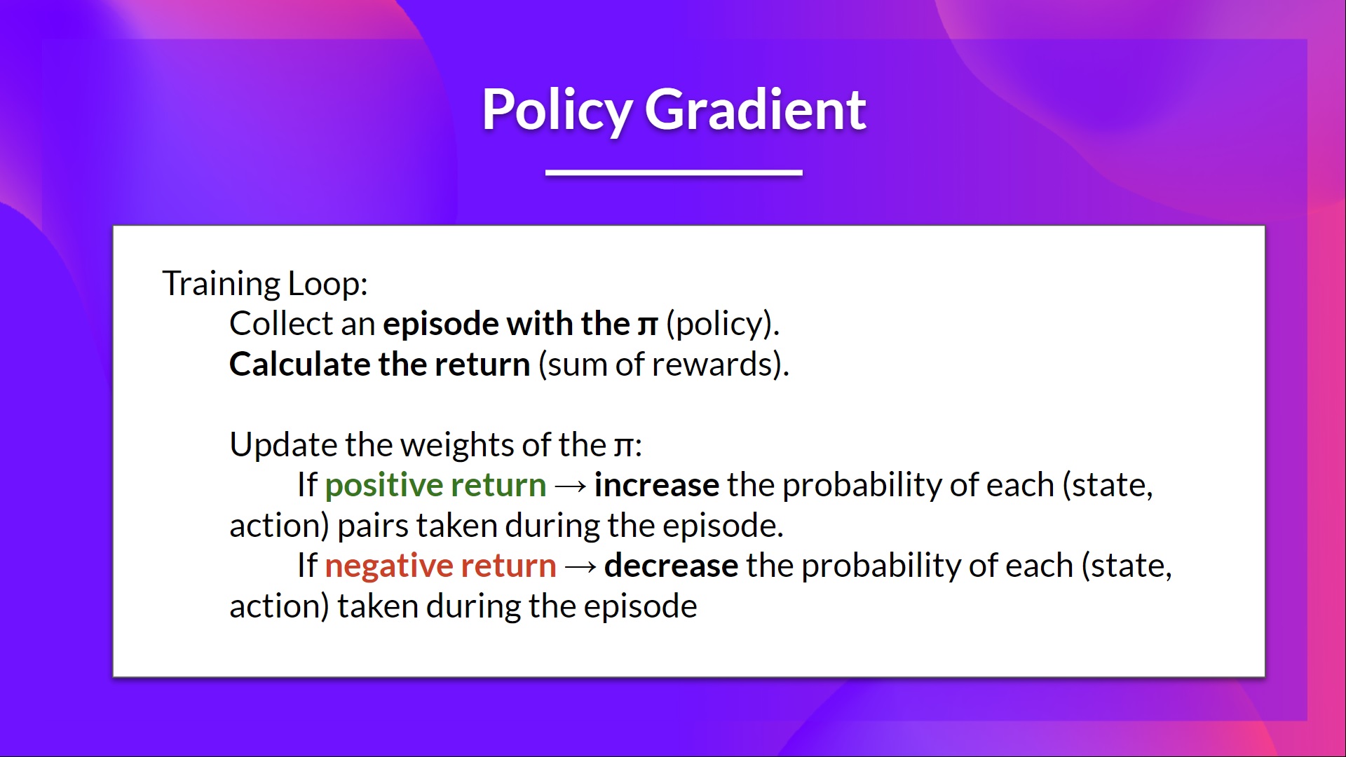
We collect an episode by letting our policy interact with its environment.
-
We then take a look at the sum of rewards of the episode (expected return). If this sum is positive, we consider that the actions taken throughout the episodes were good: Subsequently, we wish to extend the P(a|s) (probability of taking that motion at that state) for every state-action pair.
The Policy Gradient algorithm (simplified) looks like this:
But Deep Q-Learning is great! Why use policy gradient methods?
The Benefits of Policy-Gradient Methods
There are multiple benefits over Deep Q-Learning methods. Let’s have a look at a few of them:
-
The simplicity of the mixing: we are able to estimate the policy directly without storing additional data (motion values).
-
Policy gradient methods can learn a stochastic policy while value functions cannot.
This has two consequences:
a. We need not implement an exploration/exploitation trade-off by hand. Since we output a probability distribution over actions, the agent explores the state space without all the time taking the identical trajectory.
b. We also eliminate the issue of perceptual aliasing. Perceptual aliasing is when two states seem (or are) the identical but need different actions.
Let’s take an example: we now have an intelligent vacuum cleaner whose goal is to suck the dust and avoid killing the hamsters.

Our vacuum cleaner can only perceive where the partitions are.
The issue is that the 2 red cases are aliased states since the agent perceives an upper and lower wall for every.
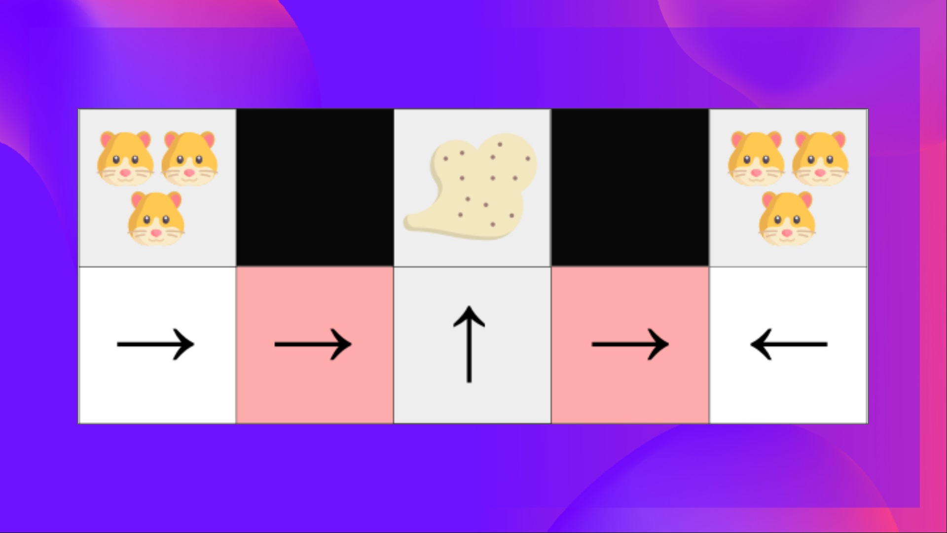
Under a deterministic policy, the policy will either move right when in a red state or move left. Either case will cause our agent to get stuck and never suck the dust.
Under a value-based RL algorithm, we learn a quasi-deterministic policy (“greedy epsilon strategy”). Consequently, our agent can spend a whole lot of time before finding the dust.
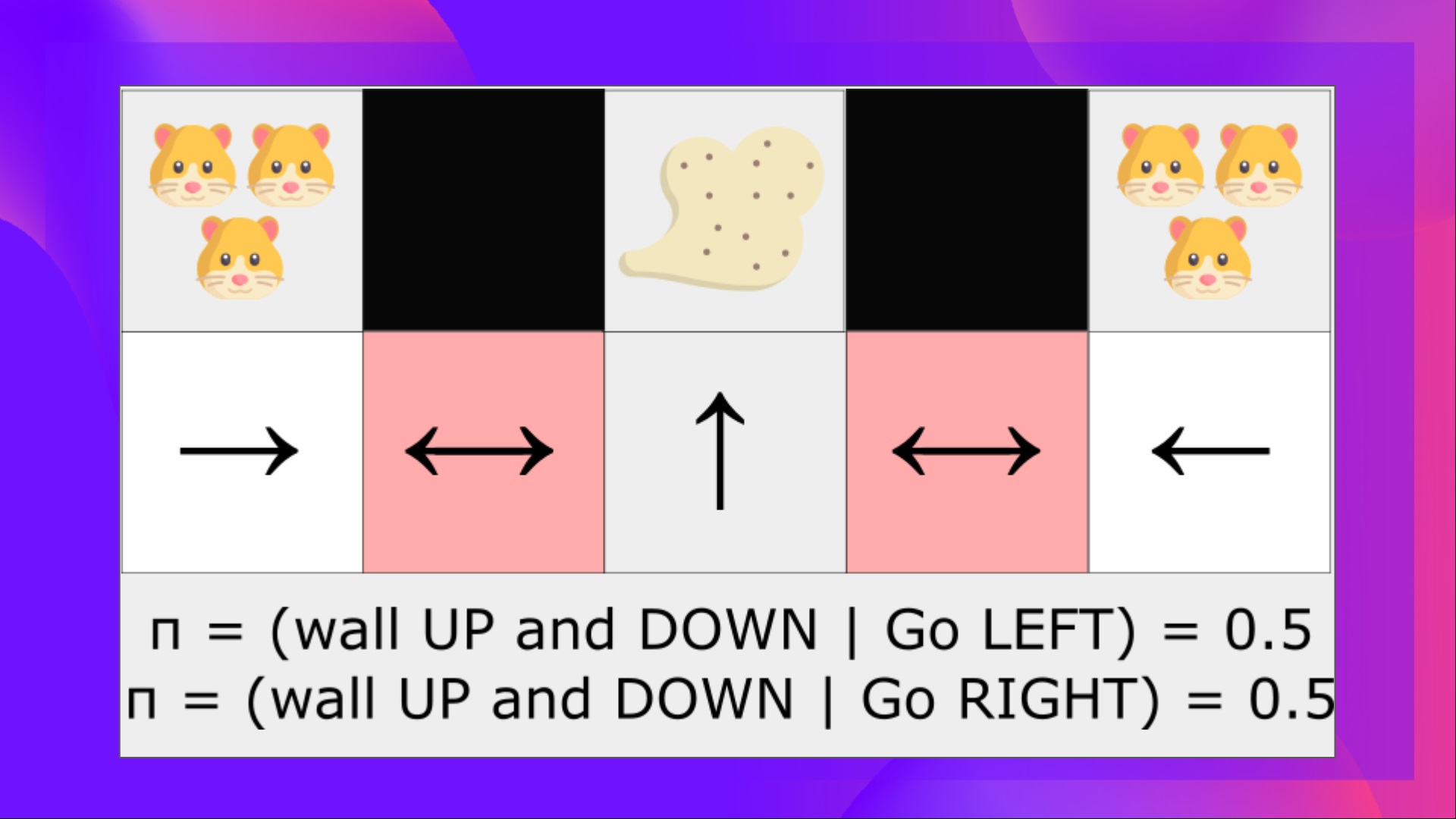
Alternatively, an optimal stochastic policy will randomly move left or right in grey states. Consequently, it’ll not be stuck and can reach the goal state with a high probability.
- Policy gradients are simpler in high-dimensional motion spaces and continuous actions spaces
Indeed, the issue with Deep Q-learning is that their predictions assign a rating (maximum expected future reward) for every possible motion, at every time step, given the present state.
But what if we now have an infinite possibility of actions?
For example, with a self-driving automotive, at each state, you’ll be able to have a (near) infinite alternative of actions (turning the wheel at 15°, 17.2°, 19,4°, honking, etc.). We’ll must output a Q-value for every possible motion! And taking the max motion of a continuous output is an optimization problem itself!
As an alternative, with a policy gradient, we output a probability distribution over actions.
The Disadvantages of Policy-Gradient Methods
Naturally, Policy Gradient methods have also some disadvantages:
- Policy gradients converge a whole lot of time on an area maximum as an alternative of a worldwide optimum.
- Policy gradient goes faster, step-by-step: it will probably take longer to coach (inefficient).
- Policy gradient can have high variance (solution baseline).
👉 If you desire to go deeper on the why the benefits and downsides of Policy Gradients methods, you’ll be able to check this video.
Now that we now have seen the large picture of Policy-Gradient and its benefits and downsides, let’s study and implement one among them: Reinforce.
Reinforce (Monte Carlo Policy Gradient)
Reinforce, also called Monte-Carlo Policy Gradient, uses an estimated return from a complete episode to update the policy parameter .
We’ve our policy π which has a parameter θ. This π, given a state, outputs a probability distribution of actions.
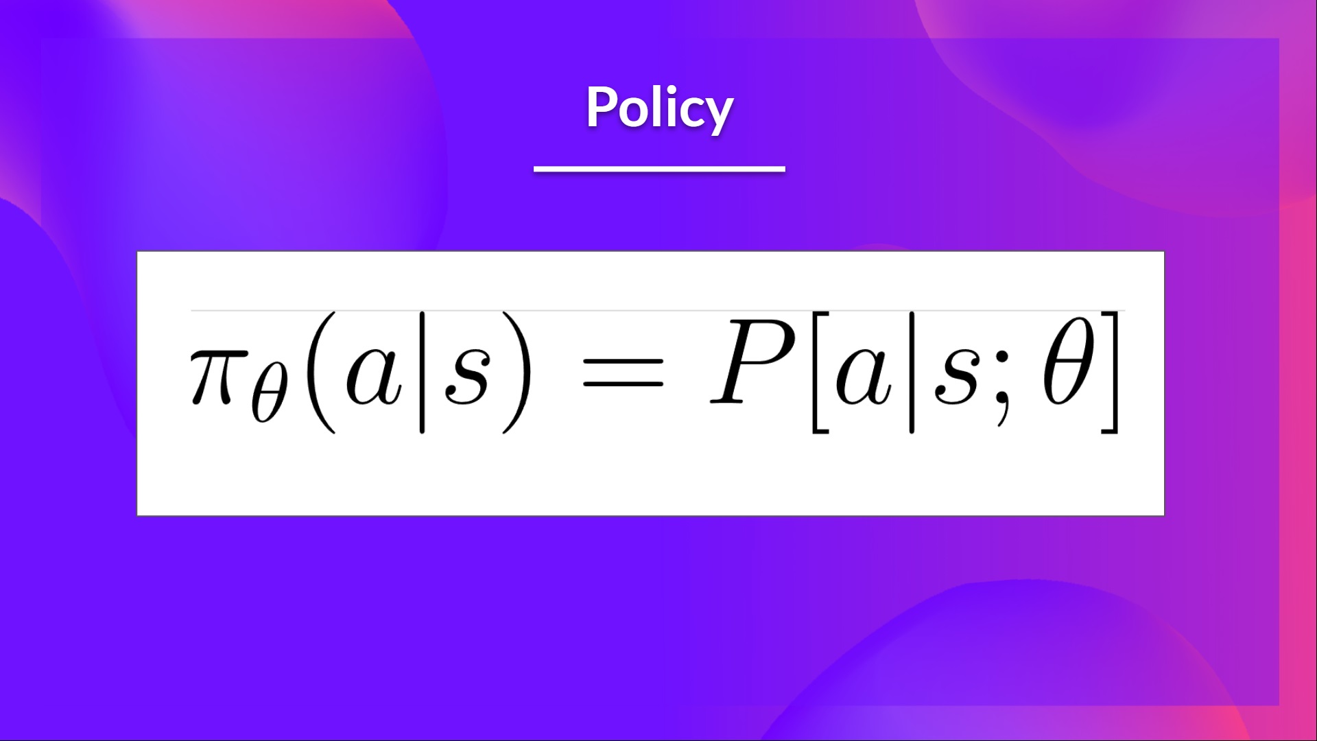
Where is the probability of the agent choosing motion at from state st, given our policy.
But how can we know if our policy is sweet? We’d like to have a strategy to measure it. To know that we define a rating/objective function called .
The rating function J is the expected return:
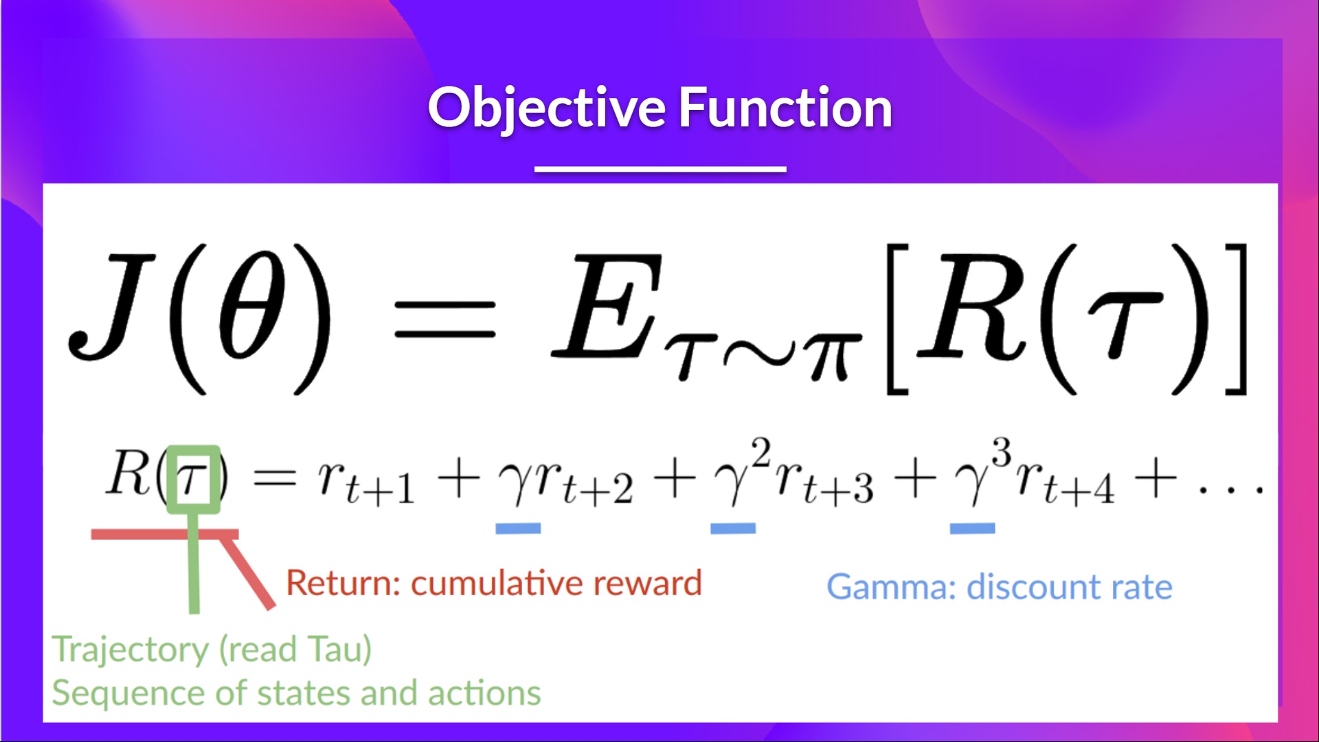
Keep in mind that policy gradient may be seen as an optimization problem. So we must find the very best parameters (θ) to maximise the rating function, J(θ).
To try this we’re going to make use of the Policy Gradient Theorem. I’m not going to dive on the mathematical details but in the event you’re interested check this video
The Reinforce algorithm works like this:
Loop:
- Use the policy to gather an episode
- Use the episode to estimate the gradient
- Update the weights of the policy:
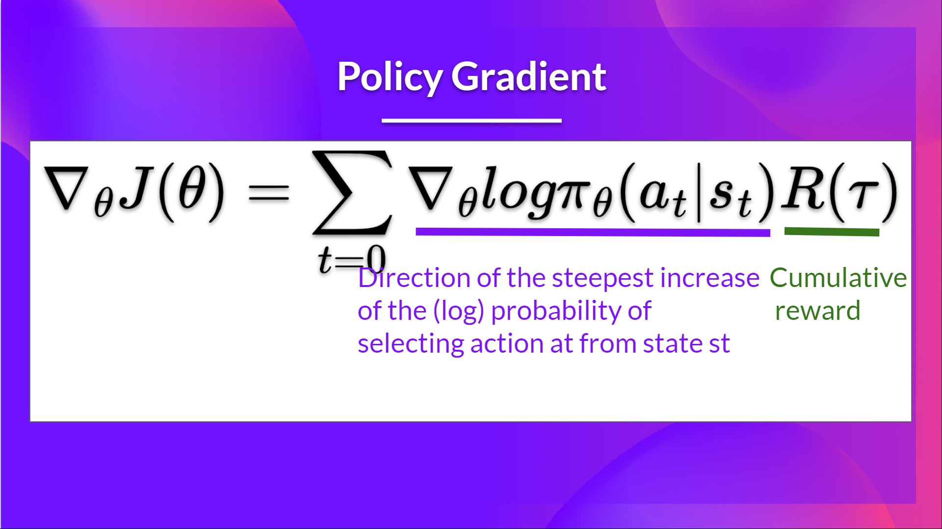
The interpretation we are able to make is that this one:
- is the direction of steepest increase of the (log) probability of choosing motion at from state st.
=> This tells use how we should always change the weights of policy if we wish to extend/decrease the log probability of choosing motion at at state st. - : is the scoring function:
- If the return is high, it’ll push up the chances of the (state, motion) combos.
- Else, if the return is low, it’ll push down the chances of the (state, motion) combos.
Congrats on ending this chapter! There was a whole lot of information. And congrats on ending the tutorial. You’ve just coded your first Deep Reinforcement Learning agent from scratch using PyTorch and shared it on the Hub 🥳.
It’s normal in the event you still feel confused with all these elements. This was the identical for me and for all individuals who studied RL.
Take time to actually grasp the fabric before continuing.
Don’t hesitate to coach your agent in other environments. The best strategy to learn is to try things on your personal!
We published additional readings within the syllabus if you desire to go deeper 👉 https://github.com/huggingface/deep-rl-class/blob/primary/unit5/README.md
In the subsequent unit, we’re going to study a mixture of Policy-Based and Value-based methods called Actor Critic Methods.
And do not forget to share with your pals who wish to learn 🤗!
Finally, we wish to enhance and update the course iteratively together with your feedback. If you could have some, please fill this kind 👉 https://forms.gle/3HgA7bEHwAmmLfwh9