

In recent times, training ever larger language models has develop into the norm. While the problems of those models’ not being released for further study is often discussed, the hidden knowledge about how one can train such models rarely gets any attention. This text goals to vary this by shedding some light on the technology and engineering behind training such models each when it comes to hardware and software on the instance of the 176B parameter language model BLOOM.
But first we would love to thank the businesses and key people and groups that made the amazing feat of coaching a 176 Billion parameter model by a small group of dedicated people possible.
Then the hardware setup and fundamental technological components might be discussed.

Here’s a fast summary of project:
| Hardware | 384 80GB A100 GPUs |
| Software | Megatron-DeepSpeed |
| Architecture | GPT3 w/ extras |
| Dataset | 350B tokens of 59 Languages |
| Training time | 3.5 months |
People
The project was conceived by Thomas Wolf (co-founder and CSO – Hugging Face), who dared to compete with the large corporations not only to coach considered one of the most important multilingual models, but in addition to make the end result accessible to all people, thus making what was but a dream to most individuals a reality.
This text focuses specifically on the engineering side of the training of the model. A very powerful a part of the technology behind BLOOM were the people and corporations who shared their expertise and helped us with coding and training.
There are 6 fundamental groups of individuals to thank:
- The HuggingFace’s BigScience team who dedicated greater than half a dozen full time employees to work out and run the training from inception to the ending line and provided and paid for all of the infrastructure beyond the Jean Zay’s compute.
- The Microsoft DeepSpeed team, who developed DeepSpeed and later integrated it with Megatron-LM, and whose developers spent many weeks working on the needs of the project and provided plenty of awesome practical experiential advice before and throughout the training.
- The NVIDIA Megatron-LM team, who developed Megatron-LM and who were super helpful answering our quite a few questions and providing firstclass experiential advice.
- The IDRIS / GENCI team managing the Jean Zay supercomputer, who donated to the project an insane amount of compute and great system administration support.
- The PyTorch team who created a brilliant powerful framework, on which the remainder of the software was based, and who were very supportive to us throughout the preparation for the training, fixing multiple bugs and improving the usability of the PyTorch components we relied on throughout the training.
- The volunteers within the BigScience Engineering workgroup
It would be very difficult to call all of the amazing individuals who contributed to the engineering side of the project, so I’ll just name a number of key people outside of Hugging Face who were the engineering foundation of this project for the last 14 months:
Olatunji Ruwase, Deepak Narayanan, Jeff Rasley, Jared Casper, Samyam Rajbhandari and Rémi Lacroix
Also we’re grateful to all the businesses who allowed their employees to contribute to this project.
Overview
BLOOM’s architecture could be very just like GPT3 with a number of added improvements as might be discussed later in this text.
The model was trained on Jean Zay, the French government-funded super computer that’s managed by GENCI and installed at IDRIS, the national computing center for the French National Center for Scientific Research (CNRS). The compute was generously donated to the project by GENCI (grant 2021-A0101012475).
The next hardware was used throughout the training:
- GPUs: 384 NVIDIA A100 80GB GPUs (48 nodes) + 32 spare gpus
- 8 GPUs per node Using NVLink 4 inter-gpu connects, 4 OmniPath links
- CPU: AMD EPYC 7543 32-Core Processor
- CPU memory: 512GB per node
- GPU memory: 640GB per node
- Inter-node connect: Omni-Path Architecture (OPA) w/ non-blocking fat tree
- NCCL-communications network: a completely dedicated subnet
- Disc IO network: GPFS shared with other nodes and users
Checkpoints:
- fundamental checkpoints
- each checkpoint with fp32 optim states and bf16+fp32 weights is 2.3TB – just the bf16 weights are 329GB.
Datasets:
The training of the 176B BLOOM model occurred over Mar-Jul 2022 and took about 3.5 months to finish (roughly 1M compute hours).
Megatron-DeepSpeed
The 176B BLOOM model has been trained using Megatron-DeepSpeed, which is a mix of two fundamental technologies:
- DeepSpeed is a deep learning optimization library that makes distributed training easy, efficient, and effective.
- Megatron-LM is a big, powerful transformer model framework developed by the Applied Deep Learning Research team at NVIDIA.
The DeepSpeed team developed a 3D parallelism based implementation by combining ZeRO sharding and pipeline parallelism from the DeepSpeed library with Tensor Parallelism from Megatron-LM. More details about each component may be seen within the table below.
Please note that the BigScience’s Megatron-DeepSpeed is a fork of the unique Megatron-DeepSpeed repository, to which we added multiple additions.
Here’s a table of which components were provided by which framework to coach BLOOM:
Please note that each Megatron-LM and DeepSpeed have Pipeline Parallelism and BF16 Optimizer implementations, but we used those from DeepSpeed as they’re integrated with ZeRO.
Megatron-DeepSpeed implements 3D Parallelism to permit huge models to coach in a really efficient way. Let’s briefly discuss the 3D components.
- DataParallel (DP) – the identical setup is replicated multiple times, and every being fed a slice of the info. The processing is finished in parallel and all setups are synchronized at the top of every training step.
- TensorParallel (TP) – each tensor is split up into multiple chunks, so as an alternative of getting the entire tensor reside on a single GPU, each shard of the tensor resides on its designated GPU. During processing each shard gets processed individually and in parallel on different GPUs and the outcomes are synced at the top of the step. That is what one may call horizontal parallelism, because the splitting happens on a horizontal level.
- PipelineParallel (PP) – the model is split up vertically (layer-level) across multiple GPUs, in order that just one or several layers of the model are placed on a single GPU. Each GPU processes in parallel different stages of the pipeline and works on a small chunk of the batch.
- Zero Redundancy Optimizer (ZeRO) – also performs sharding of the tensors somewhat just like TP, except the entire tensor gets reconstructed in time for a forward or backward computation, due to this fact the model doesn’t should be modified. It also supports various offloading techniques to compensate for limited GPU memory.
Data Parallelism
Most users with just a number of GPUs are more likely to be acquainted with DistributedDataParallel (DDP) PyTorch documentation. On this method the model is fully replicated to every GPU after which after each iteration all of the models synchronize their states with one another. This approach allows training speed up but throwing more resources at the issue, nevertheless it only works if the model can fit onto a single GPU.
ZeRO Data Parallelism
ZeRO-powered data parallelism (ZeRO-DP) is described on the next diagram from this blog post
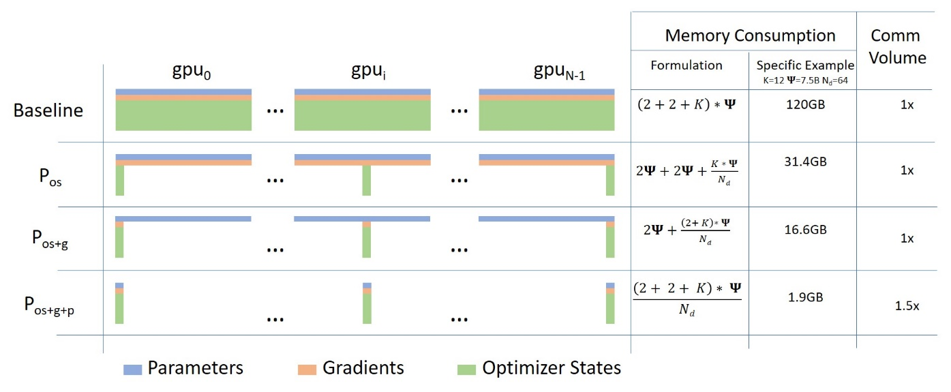
It may possibly be difficult to wrap one’s head around it, but in point of fact, the concept is sort of easy. That is just the same old DDP, except, as an alternative of replicating the total model params, gradients and optimizer states, each GPU stores only a slice of it. After which at run-time when the total layer params are needed only for the given layer, all GPUs synchronize to present one another parts that they miss – that is it.
This component is implemented by DeepSpeed.
Tensor Parallelism
In Tensor Parallelism (TP) each GPU processes only a slice of a tensor and only aggregates the total tensor for operations that require the entire thing.
On this section we use concepts and diagrams from the Megatron-LM paper: Efficient Large-Scale Language Model Training on GPU Clusters.
The fundamental constructing block of any transformer is a completely connected nn.Linear followed by a nonlinear activation GeLU.
Following the Megatron paper’s notation, we are able to write the dot-product a part of it as Y = GeLU(XA), where X and Y are the input and output vectors, and A is the load matrix.
If we have a look at the computation in matrix form, it is simple to see how the matrix multiplication may be split between multiple GPUs:
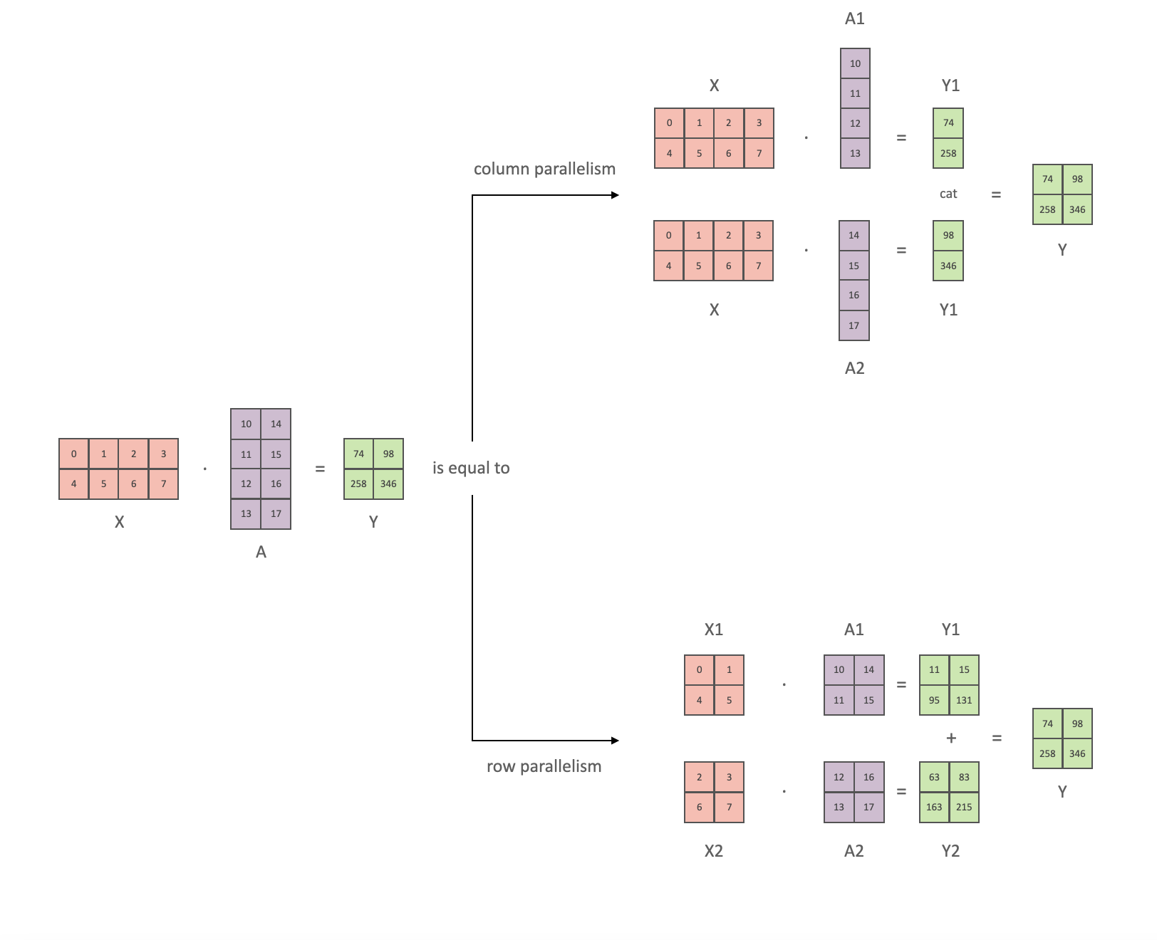
If we split the load matrix A column-wise across N GPUs and perform matrix multiplications XA_1 through XA_n in parallel, then we are going to find yourself with N output vectors Y_1, Y_2, ..., Y_n which may be fed into GeLU independently:
 . Notice with the Y matrix split along the columns, we are able to split the second GEMM along its rows in order that it takes the output of the GeLU directly with none extra communication.
Using this principle, we are able to update an MLP of arbitrary depth, while synchronizing the GPUs after each row-column sequence. The Megatron-LM paper authors provide a helpful illustration for that:
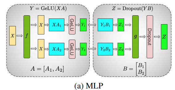
Here f is an identity operator within the forward pass and all reduce within the backward pass while g is an all reduce within the forward pass and identity within the backward pass.
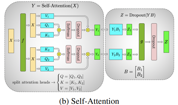
Parallelizing the multi-headed attention layers is even simpler, since they’re already inherently parallel, attributable to having multiple independent heads!
Special considerations: On account of the 2 all reduces per layer in each the forward and backward passes, TP requires a really fast interconnect between devices. Subsequently it isn’t advisable to do TP across a couple of node, unless you’ve got a really fast network. In our case the inter-node was much slower than PCIe. Practically, if a node has 4 GPUs, the best TP degree is due to this fact 4. In case you need a TP degree of 8, you’ll want to use nodes which have not less than 8 GPUs.
This component is implemented by Megatron-LM. Megatron-LM has recently expanded tensor parallelism to incorporate sequence parallelism that splits the operations that can’t be split as above, similar to LayerNorm, along the sequence dimension. The paper Reducing Activation Recomputation in Large Transformer Models provides details for this system. Sequence parallelism was developed after BLOOM was trained so not utilized in the BLOOM training.
Pipeline Parallelism
Naive Pipeline Parallelism (naive PP) is where one spreads groups of model layers across multiple GPUs and easily moves data along from GPU to GPU as if it were one large composite GPU. The mechanism is comparatively easy – switch the specified layers .to() the specified devices and now at any time when the info goes out and in those layers switch the info to the identical device because the layer and leave the remainder unmodified.
This performs a vertical model parallelism, because if you happen to remember how most models are drawn, we slice the layers vertically. For instance, if the next diagram shows an 8-layer model:
===================  ===================
|  0 | 1 | 2 | 3  |  |  4 | 5 | 6 | 7  |
===================  ===================
        GPU0                 GPU1
we just sliced it in 2 vertically, placing layers 0-3 onto GPU0 and 4-7 to GPU1.
Now while data travels from layer 0 to 1, 1 to 2 and a couple of to three that is similar to the forward pass of a traditional model on a single GPU. But when data must pass from layer 3 to layer 4 it must travel from GPU0 to GPU1 which introduces a communication overhead. If the participating GPUs are on the identical compute node (e.g. same physical machine) this copying is pretty fast, but when the GPUs are situated on different compute nodes (e.g. multiple machines) the communication overhead could possibly be significantly larger.
Then layers 4 to five to six to 7 are as a traditional model would have and when the seventh layer completes we regularly must send the info back to layer 0 where the labels are (or alternatively send the labels to the last layer). Now the loss may be computed and the optimizer can do its work.
Problems:
- the fundamental deficiency and why this one is named “naive” PP, is that each one but one GPU is idle at any given moment. So if 4 GPUs are used, it’s almost an identical to quadrupling the quantity of memory of a single GPU, and ignoring the remainder of the hardware. Plus there’s the overhead of copying the info between devices. So 4x 6GB cards will have the option to accommodate the identical size as 1x 24GB card using naive PP, except the latter will complete the training faster, because it doesn’t have the info copying overhead. But, say, if you’ve got 40GB cards and want to suit a 45GB model you’ll be able to with 4x 40GB cards (but barely due to gradient and optimizer states).
- shared embeddings may have to get copied forwards and backwards between GPUs.
Pipeline Parallelism (PP) is sort of an identical to a naive PP described above, nevertheless it solves the GPU idling problem, by chunking the incoming batch into micro-batches and artificially making a pipeline, which allows different GPUs to concurrently take part in the computation process.
The next illustration from the GPipe paper shows the naive PP on the highest, and PP on the underside:
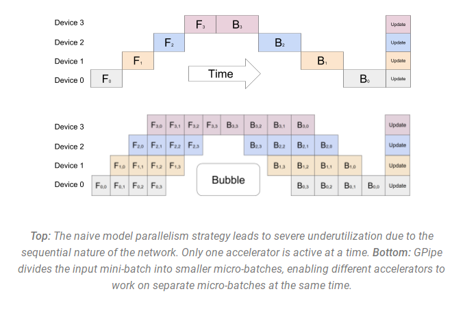
It is simple to see from the underside diagram how PP has fewer dead zones, where GPUs are idle. The idle parts are known as the “bubble”.
Each parts of the diagram show parallelism that’s of degree 4. That’s 4 GPUs are participating within the pipeline. So there’s the forward path of 4 pipe stages F0, F1, F2 and F3 after which the return reverse order backward path of B3, B2, B1 and B0.
PP introduces a brand new hyper-parameter to tune that is named chunks. It defines what number of chunks of information are sent in a sequence through the identical pipe stage. For instance, in the underside diagram, you’ll be able to see that chunks=4. GPU0 performs the identical forward path on chunk 0, 1, 2 and three (F0,0, F0,1, F0,2, F0,3) after which it waits for other GPUs to do their work and only when their work is beginning to be complete, does GPU0 begin to work again doing the backward path for chunks 3, 2, 1 and 0 (B0,3, B0,2, B0,1, B0,0).
Note that conceptually this is identical concept as gradient accumulation steps (GAS). PyTorch uses chunks, whereas DeepSpeed refers back to the same hyper-parameter as GAS.
Due to the chunks, PP introduces the concept of micro-batches (MBS). DP splits the worldwide data batch size into mini-batches, so if you’ve got a DP degree of 4, a world batch size of 1024 gets split up into 4 mini-batches of 256 each (1024/4). And if the variety of chunks (or GAS) is 32 we find yourself with a micro-batch size of 8 (256/32). Each Pipeline stage works with a single micro-batch at a time.
To calculate the worldwide batch size of the DP + PP setup we then do: mbs*chunks*dp_degree (8*32*4=1024).
Let’s return to the diagram.
With chunks=1 you find yourself with the naive PP, which could be very inefficient. With a really large chunks value you find yourself with tiny micro-batch sizes which could possibly be not very efficient either. So one has to experiment to search out the worth that results in the best efficient utilization of the GPUs.
While the diagram shows that there’s a bubble of “dead” time that cannot be parallelized since the last forward stage has to attend for backward to finish the pipeline, the aim of finding the perfect value for chunks is to enable a high concurrent GPU utilization across all participating GPUs which translates to minimizing the scale of the bubble.
This scheduling mechanism is often called all forward all backward. Another alternatives are one forward one backward and interleaved one forward one backward.
While each Megatron-LM and DeepSpeed have their very own implementation of the PP protocol, Megatron-DeepSpeed uses the DeepSpeed implementation because it’s integrated with other facets of DeepSpeed.
One other necessary issue here is the scale of the word embedding matrix. While normally a word embedding matrix consumes less memory than the transformer block, in our case with an enormous 250k vocabulary, the embedding layer needed 7.2GB in bf16 weights and the transformer block is just 4.9GB. Subsequently, we needed to instruct Megatron-Deepspeed to think about the embedding layer as a transformer block. So we had a pipeline of 72 layers, 2 of which were dedicated to the embedding (first and last). This allowed to balance out the GPU memory consumption. If we didn’t do it, we might have had the primary and the last stages devour a lot of the GPU memory, and 95% of GPUs could be using much less memory and thus the training could be removed from being efficient.
DP+PP
The next diagram from the DeepSpeed pipeline tutorial demonstrates how one combines DP with PP.
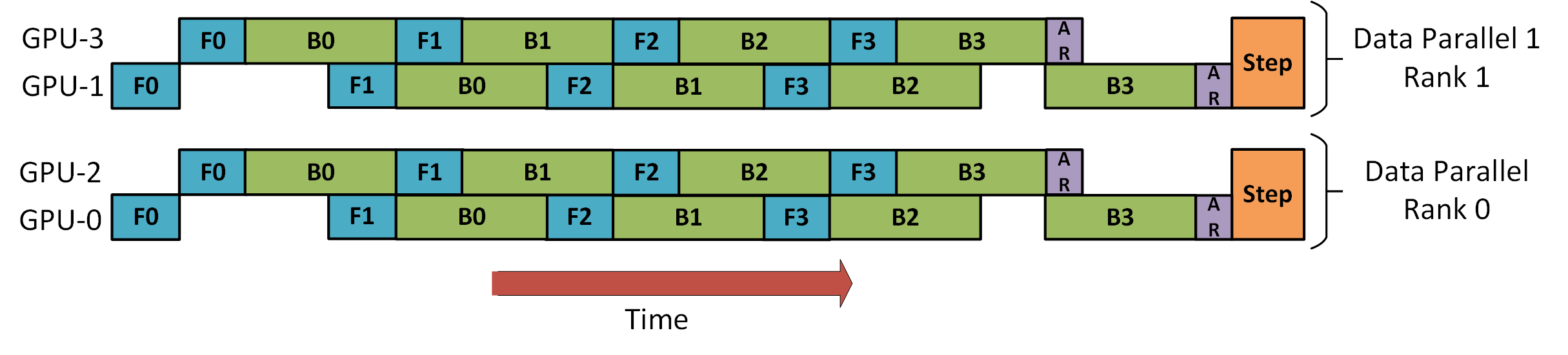
Here it is important to see how DP rank 0 doesn’t see GPU2 and DP rank 1 doesn’t see GPU3. To DP there are only GPUs 0 and 1 where it feeds data as if there have been just 2 GPUs. GPU0 “secretly” offloads a few of its load to GPU2 using PP. And GPU1 does the identical by enlisting GPU3 to its aid.
Since each dimension requires not less than 2 GPUs, here you’d need not less than 4 GPUs.
DP+PP+TP
To get a good more efficient training PP is combined with TP and DP which is named 3D parallelism. This may be seen in the next diagram.
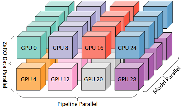
This diagram is from a blog post 3D parallelism: Scaling to trillion-parameter models, which is a very good read as well.
Since each dimension requires not less than 2 GPUs, here you’d need not less than 8 GPUs for full 3D parallelism.
ZeRO DP+PP+TP
One among the fundamental features of DeepSpeed is ZeRO, which is a super-scalable extension of DP. It has already been discussed in ZeRO Data Parallelism. Normally it is a standalone feature that does not require PP or TP. But it may be combined with PP and TP.
When ZeRO-DP is combined with PP (and optionally TP) it typically enables only ZeRO stage 1, which shards only optimizer states. ZeRO stage 2 moreover shards gradients, and stage 3 also shards the model weights.
While it’s theoretically possible to make use of ZeRO stage 2 with Pipeline Parallelism, it would have bad performance impacts. There would should be an extra reduce-scatter collective for each micro-batch to aggregate the gradients before sharding, which adds a potentially significant communication overhead. By nature of Pipeline Parallelism, small micro-batches are used and as an alternative the main focus is on attempting to balance arithmetic intensity (micro-batch size) with minimizing the Pipeline bubble (variety of micro-batches). Subsequently those communication costs are going to harm.
As well as, there are already fewer layers than normal attributable to PP and so the memory savings won’t be huge. PP already reduces gradient size by 1/PP, and so gradient sharding savings on top of which are less important than pure DP.
ZeRO stage 3 may also be used to coach models at this scale, nonetheless, it requires more communication than the DeepSpeed 3D parallel implementation. After careful evaluation in our surroundings which happened a 12 months ago we found Megatron-DeepSpeed 3D parallelism performed best. Since then ZeRO stage 3 performance has dramatically improved and if we were to guage it today perhaps we might have chosen stage 3 as an alternative.
BF16Optimizer
Training huge LLM models in FP16 is a no-no.
We’ve proved it to ourselves by spending several months training a 104B model which as you’ll be able to tell from the tensorboard was but a whole failure. We learned a whole lot of things while fighting the ever diverging lm-loss:
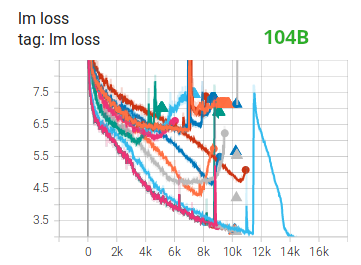
and we also got the identical advice from the Megatron-LM and DeepSpeed teams after they trained the 530B model. The recent release of OPT-175B too reported that that they had a really difficult time training in FP16.
So back in January as we knew we could be training on A100s which support the BF16 format Olatunji Ruwase developed a BF16Optimizer which we used to coach BLOOM.
In case you aren’t acquainted with this data format, please take a look on the bits layout. The important thing to BF16 format is that it has the identical exponent as FP32 and thus doesn’t suffer from overflow FP16 suffers from quite a bit! With FP16, which has a max numerical range of 64k, you’ll be able to only multiply small numbers. e.g. you’ll be able to do 250*250=62500, but if you happen to were to try 255*255=65025 you bought yourself an overflow, which is what causes the fundamental problems during training. This implies your weights should remain tiny. A method called loss scaling may help with this problem, however the limited range of FP16 remains to be a problem when models develop into very large.
BF16 has no such problem, you’ll be able to easily do 10_000*10_000=100_000_000 and it’s no problem.
In fact, since BF16 and FP16 have the identical size of two bytes, one doesn’t get a free lunch and one pays with really bad precision when using BF16. Nonetheless, if you happen to remember the training using stochastic gradient descent and its variations is a type of stumbling walk, so if you happen to do not get the proper direction immediately it’s no problem, you’ll correct yourself in the subsequent steps.
No matter whether one uses BF16 or FP16 there’s also a duplicate of weights which is all the time in FP32 – that is what gets updated by the optimizer. So the 16-bit formats are only used for the computation, the optimizer updates the FP32 weights with full precision after which casts them into the 16-bit format for the subsequent iteration.
All PyTorch components have been updated to make sure that they perform any accumulation in FP32, so no loss happening there.
One crucial issue is gradient accumulation, and it’s considered one of the fundamental features of pipeline parallelism because the gradients from each microbatch processing get collected. It’s crucial to implement gradient accumulation in FP32 to maintain the training precise, and that is what BF16Optimizer does.
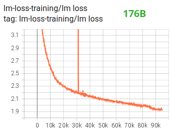
Besides other improvements we imagine that using BF16 mixed precision training turned a possible nightmare into a comparatively smooth process which may be observed from the next lm loss graph:
Fused CUDA Kernels
The GPU performs two things. It may possibly copy data to/from memory and perform computations on that data. While the GPU is busy copying the GPU’s computations units idle. If we would like to efficiently utilize the GPU we would like to attenuate the idle time.
A kernel is a set of instructions that implements a selected PyTorch operation. For instance, whenever you call torch.add, it goes through a PyTorch dispatcher which looks on the input tensor(s) and various other things and decides which code it should run, after which runs it. A CUDA kernel is a selected implementation that uses the CUDA API library and might only run on NVIDIA GPUs.
Now, when instructing the GPU to compute c = torch.add(a, b); e = torch.max([c,d]), a naive approach, and what PyTorch will do unless instructed otherwise, is to launch two separate kernels, one to perform the addition of a and b and one other to search out the utmost value between c and d. On this case, the GPU fetches from its memory a and b, performs the addition, after which copies the result back into the memory. It then fetches c and d and performs the max operation and again copies the result back into the memory.
If we were to fuse these two operations, i.e. put them right into a single “fused kernel”, and just launch that one kernel we can’t copy the intermediary result c to the memory, but leave it within the GPU registers and only must fetch d to finish the last computation. This protects a whole lot of overhead and prevents GPU idling and makes the entire operation far more efficient.
Fused kernels are only that. Primarily they replace multiple discrete computations and data movements to/from memory into fused computations which have only a few memory movements. Moreover, some fused kernels rewrite the mathematics in order that certain groups of computations may be performed faster.
To coach BLOOM fast and efficiently it was essential to make use of several custom fused CUDA kernels provided by Megatron-LM. Particularly there’s an optimized kernel to perform LayerNorm in addition to kernels to fuse various combos of the scaling, masking, and softmax operations. The addition of a bias term can be fused with the GeLU operation using PyTorch’s JIT functionality. These operations are all memory certain, so it is vital to fuse them to maximise the quantity of computation done once a worth has been retrieved from memory. So, for instance, adding the bias term while already doing the memory certain GeLU operation adds no additional time. These kernels are all available within the Megatron-LM repository.
Datasets
One other necessary feature from Megatron-LM is the efficient data loader. During begin of the initial training each data set is split into samples of the requested sequence length (2048 for BLOOM) and index is created to number each sample. Based on the training parameters the variety of epochs for a dataset is calculated and an ordering for that many epochs is created after which shuffled. For instance, if a dataset has 10 samples and needs to be undergone twice, the system first lays out the samples indices so as [0, ..., 9, 0, ..., 9] after which shuffles that order to create the ultimate global order for the dataset. Notice that which means that training is not going to simply undergo your complete dataset after which repeat, it is feasible to see the identical sample twice before seeing one other sample in any respect, but at the top of coaching the model may have seen each sample twice. This helps ensure a smooth training curve through your complete training process. These indices, including the offsets into the bottom dataset of every sample, are saved to a file to avoid recomputing them every time a training process is began. Several of those datasets can then be blended with various weights into the ultimate data seen by the training process.
Embedding LayerNorm
While we were fighting with attempting to stop 104B from diverging we discovered that adding an extra LayerNorm right after the primary word embedding made the training far more stable.
This insight got here from experimenting with bitsandbytes which incorporates a StableEmbedding which is a traditional Embedding with layernorm and it uses a uniform xavier initialization.
Positional Encoding
We also replaced the same old positional embedding with an AliBi – based on the paper: Train Short, Test Long: Attention with Linear Biases Enables Input Length Extrapolation, which allows to extrapolate for longer input sequences than those the model was trained on. So regardless that we train on sequences with length 2048 the model may also cope with for much longer sequences during inference.
Training Difficulties
With the architecture, hardware and software in place we were capable of start training in early March 2022. Nonetheless, it was not only smooth sailing from there. On this section we discuss among the fundamental hurdles we encountered.
There have been a whole lot of issues to work out before the training began. Particularly we found several issues that manifested themselves just once we began training on 48 nodes, and won’t appear at small scale. E.g., CUDA_LAUNCH_BLOCKING=1 was needed to stop the framework from hanging, and we wanted to separate the optimizer groups into smaller groups, otherwise the framework would again hang. You may examine those intimately within the training prequel chronicles.
The fundamental form of issue encountered during training were hardware failures. As this was a brand new cluster with about 400 GPUs, on average we were getting 1-2 GPU failures every week. We were saving a checkpoint every 3h (100 iterations) so on average we might lose 1.5h of coaching on hardware crash. The Jean Zay sysadmins would then replace the faulty GPUs and produce the node back up. Meanwhile we had backup nodes to make use of as an alternative.
We’ve run into quite a lot of other problems that led to 5-10h downtime several times, some related to a deadlock bug in PyTorch, others attributable to running out of disk space. In case you are interested by specific details please see training chronicles.
We were planning for all these downtimes when deciding on the feasibility of coaching this model – we selected the scale of the model to match that feasibility and the quantity of information we wanted the model to devour. With all of the downtimes we managed to complete the training in our estimated time. As mentioned earlier it took about 1M compute hours to finish.
One other issue was that SLURM wasn’t designed to be utilized by a team of individuals. A SLURM job is owned by a single user and if they don’t seem to be around, the opposite members of the group cannot do anything to the running job. We developed a kill-switch workaround that allowed other users within the group to kill the present process without requiring the user who began the method to be present. This worked well in 90% of the problems. If SLURM designers read this – please add an idea of Unix groups, in order that a SLURM job may be owned by a bunch.
Because the training was happening 24/7 we wanted someone to be on call – but since we had people each in Europe and West Coast Canada overall there was no need for somebody to hold a pager, we might just overlap nicely. In fact, someone had to look at the training on the weekends as well. We automated most things, including recovery from hardware crashes, but sometimes a human intervention was needed as well.
Conclusion
Probably the most difficult and intense a part of the training was the two months resulting in the beginning of the training. We were under a whole lot of pressure to begin training ASAP, for the reason that resources allocation was limited in time and we did not have access to A100s until the very last moment. So it was a really difficult time, considering that the BF16Optimizer was written within the last moment and we wanted to debug it and fix various bugs. And as explained within the previous section we discovered latest problems that manifested themselves just once we began training on 48 nodes, and won’t appear at small scale.
But once we sorted those out, the training itself was surprisingly smooth and without major problems. More often than not we had one person monitoring the training and only a number of times several people were involved to troubleshoot. We enjoyed great support from Jean Zay’s administration who quickly addressed most needs that emerged throughout the training.
Overall it was a super-intense but very rewarding experience.
Training large language models remains to be a difficult task, but we hope by constructing and sharing this technology within the open others can construct on top of our experience.
Resources
Essential links
Papers and Articles
We couldn’t have possibly explained every part intimately in this text, so if the technology presented here piqued your curiosity and you need to know more listed here are the papers to read:
Megatron-LM:
DeepSpeed:
Joint Megatron-LM and Deepspeeed:
ALiBi:
BitsNBytes:
- 8-bit Optimizers via Block-wise Quantization (within the context of Embedding LayerNorm but the remainder of the paper and the technology is amazing – the one reason were weren’t using the 8-bit optimizer is because we were already saving the optimizer memory with DeepSpeed-ZeRO).
Blog credits
Huge due to the next kind folks who asked good questions and helped improve the readability of the article (listed in alphabetical order):
Britney Muller,
Douwe Kiela,
Jared Casper,
Jeff Rasley,
Julien Launay,
Leandro von Werra,
Omar Sanseviero,
Stefan Schweter and
Thomas Wang.
The fundamental graphics was created by Chunte Lee.