Stable Diffusion with 🧨 Diffusers

Stable Diffusion 🎨
…using 🧨 Diffusers

Stable Diffusion is a text-to-image latent diffusion model created by the researchers and engineers from CompVis, Stability AI and LAION.
It’s trained on 512×512 images from a subset of the LAION-5B database.
LAION-5B is the biggest, freely accessible multi-modal dataset that currently exists.

On this post, we wish to point out tips on how to use Stable Diffusion with the 🧨 Diffusers library, explain how the model works and at last dive a bit deeper into how diffusers allows
one to customize the image generation pipeline.

Note: It is very beneficial to have a basic understanding of how diffusion models work. If diffusion
models are completely recent to you, we recommend reading one in every of the next blog posts:

Now, let’s start by generating some images 🎨.

Running Stable Diffusion

License

Before using the model, that you must accept the model license as a way to download and use the weights. Note: the license doesn’t must be explicitly accepted through the UI anymore.

The license is designed to mitigate the potential harmful effects of such a strong machine learning system.
We request users to read the license entirely and punctiliously. Here we provide a summary:

1. You’ll be able to’t use the model to deliberately produce nor share illegal or harmful outputs or content,
2. We claim no rights on the outputs you generate, you’re free to make use of them and are accountable for his or her use which mustn’t go against the provisions set within the license, and
3. You could re-distribute the weights and use the model commercially and/or as a service. When you do, please remember you could have to incorporate the identical use restrictions because the ones within the license and share a duplicate of the CreativeML OpenRAIL-M to all of your users.

Usage

First, it is best to install diffusers==0.10.2 to run the next code snippets:

pip install diffusers==0.10.2 transformers scipy ftfy speed up

On this post we’ll use model version v1-4, but you can even use other versions of the model similar to 1.5, 2, and a couple of.1 with minimal code changes.

The Stable Diffusion model may be run in inference with just a few lines using the StableDiffusionPipeline pipeline. The pipeline sets up every part that you must generate images from text with
a straightforward from_pretrained function call.

from diffusers import StableDiffusionPipeline

pipe = StableDiffusionPipeline.from_pretrained("CompVis/stable-diffusion-v1-4")

If a GPU is offered, let’s move it to 1!

pipe.to("cuda")

Note: When you are limited by GPU memory and have lower than 10GB of GPU RAM available, please
be sure to load the StableDiffusionPipeline in float16 precision as a substitute of the default
float32 precision as done above.

You’ll be able to achieve this by loading the weights from the fp16 branch and by telling diffusers to expect the
weights to be in float16 precision:

import torch
from diffusers import StableDiffusionPipeline

pipe = StableDiffusionPipeline.from_pretrained("CompVis/stable-diffusion-v1-4", revision="fp16", torch_dtype=torch.float16)

To run the pipeline, simply define the prompt and call pipe.

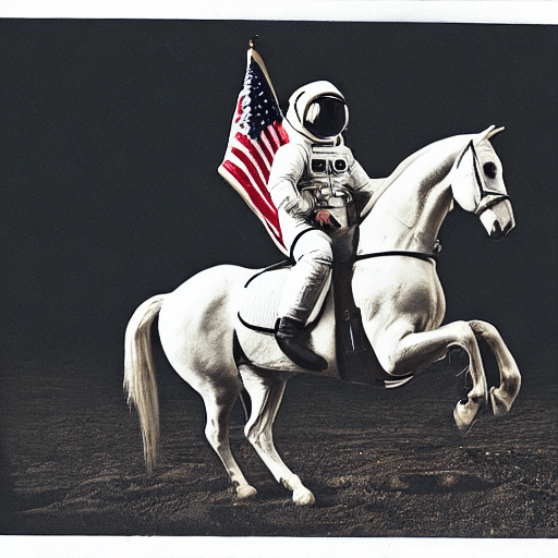
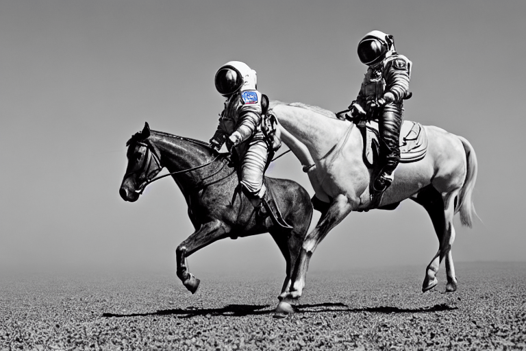
prompt = "a photograph of an astronaut riding a horse"

image = pipe(prompt).images[0]

The result would look as follows

The previous code will provide you with a distinct image each time you run it.

If sooner or later you get a black image, it could be since the content filter built contained in the model may need detected an NSFW result.
When you consider this should not be the case, try tweaking your prompt or using a distinct seed. The truth is, the model predictions include details about whether NSFW was detected for a specific result. Let’s examine what they appear like:

result = pipe(prompt)
print(result)

{
    'images': [512x512>],
    'nsfw_content_detected': [False]
}

When you want deterministic output you possibly can seed a random seed and pass a generator to the pipeline.
Each time you employ a generator with the identical seed you will get the identical image output.

import torch

generator = torch.Generator("cuda").manual_seed(1024)
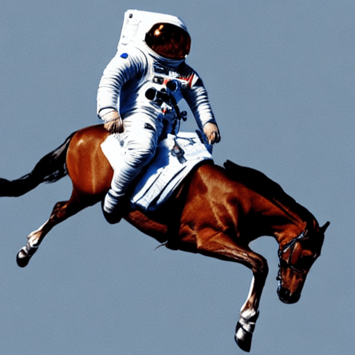
image = pipe(prompt, guidance_scale=7.5, generator=generator).images[0]

The result would look as follows

You’ll be able to change the variety of inference steps using the num_inference_steps argument.

On the whole, results are higher the more steps you employ, nevertheless the more steps, the longer the generation takes.
Stable Diffusion works quite well with a comparatively small variety of steps, so we recommend using the default variety of inference steps of 50.
When you want faster results you should use a smaller number. When you want potentially higher quality results,
you should use larger numbers.

Let’s check out running the pipeline with less denoising steps.

import torch

generator = torch.Generator("cuda").manual_seed(1024)
image = pipe(prompt, guidance_scale=7.5, num_inference_steps=15, generator=generator).images[0]

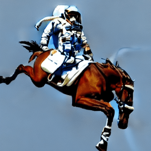
Note how the structure is similar, but there are problems within the astronauts suit and the final type of the horse.
This shows that using only 15 denoising steps has significantly degraded the standard of the generation result. As stated earlier 50 denoising steps is normally sufficient to generate high-quality images.

Besides num_inference_steps, we have been using one other function argument, called guidance_scale in all
previous examples. guidance_scale is a strategy to increase the adherence to the conditional signal that guides the generation (text, on this case) in addition to overall sample quality.
It’s also referred to as classifier-free guidance, which in easy terms forces the generation to higher match the prompt potentially at the associated fee of image quality or diversity.
Values between 7 and 8.5 are frequently good selections for Stable Diffusion. By default the pipeline
uses a guidance_scale of seven.5.

When you use a really large value the pictures might look good, but will probably be less diverse.
You’ll be able to learn concerning the technical details of this parameter in this section of the post.

Next, let’s have a look at how you possibly can generate several images of the identical prompt directly.
First, we’ll create an image_grid function to assist us visualize them nicely in a grid.

from PIL import Image

def image_grid(imgs, rows, cols):
    assert len(imgs) == rows*cols

    w, h = imgs[0].size
    grid = Image.recent('RGB', size=(cols*w, rows*h))
    grid_w, grid_h = grid.size
    
    for i, img in enumerate(imgs):
        grid.paste(img, box=(i%cols*w, i//cols*h))
    return grid

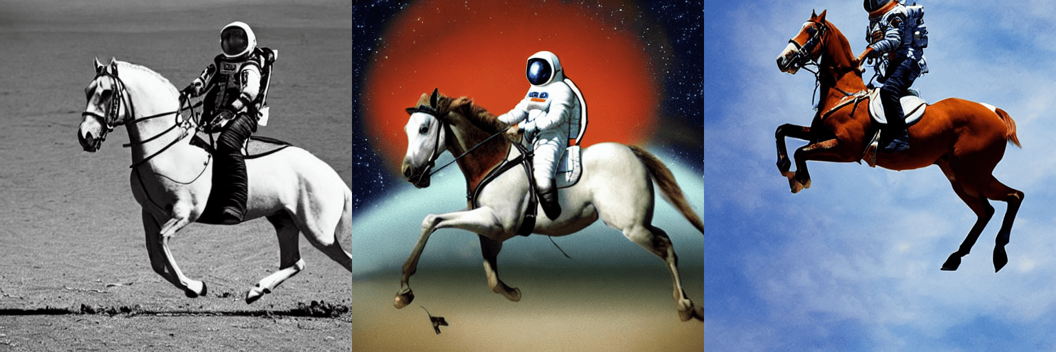
We are able to generate multiple images for a similar prompt by simply using a listing with the identical prompt repeated several times. We’ll send the list to the pipeline as a substitute of the string we used before.

num_images = 3
prompt = ["a photograph of an astronaut riding a horse"] * num_images

images = pipe(prompt).images

grid = image_grid(images, rows=1, cols=3)

By default, stable diffusion produces images of 512 × 512 pixels. It’s totally easy to override the default using the height and width arguments to create rectangular images in portrait or landscape ratios.

When selecting image sizes, we advise the next:

• Make certain height and width are each multiples of 8.
• Going below 512 might lead to lower quality images.
• Going over 512 in each directions will repeat image areas (global coherence is lost).
• One of the best strategy to create non-square images is to make use of 512 in a single dimension, and a worth larger than that in the opposite one.

Let’s run an example:

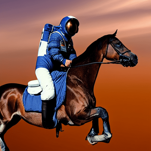
prompt = "a photograph of an astronaut riding a horse"
image = pipe(prompt, height=512, width=768).images[0]

How does Stable Diffusion work?

Having seen the high-quality images that stable diffusion can produce, let’s try to grasp
a bit higher how the model functions.

Stable Diffusion is predicated on a specific form of diffusion model called Latent Diffusion, proposed in High-Resolution Image Synthesis with Latent Diffusion Models.

Generally speaking, diffusion models are machine learning systems which can be trained to denoise random Gaussian noise step-by-step, to get to a sample of interest, similar to an image. For a more detailed overview of how they work, check this colab.

Diffusion models have shown to realize state-of-the-art results for generating image data. But one downside of diffusion models is that the reverse denoising process is slow due to its repeated, sequential nature. As well as, these models eat plenty of memory because they operate in pixel space, which becomes huge when generating high-resolution images. Subsequently, it’s difficult to coach these models and likewise use them for inference.

Latent diffusion can reduce the memory and compute complexity by applying the diffusion process over a lower dimensional latent space, as a substitute of using the actual pixel space. That is the important thing difference between standard diffusion and latent diffusion models: in latent diffusion the model is trained to generate latent (compressed) representations of the pictures.

There are three important components in latent diffusion.

1. An autoencoder (VAE).
2. A U-Net.
3. A text-encoder, e.g. CLIP’s Text Encoder.

1. The autoencoder (VAE)

The VAE model has two parts, an encoder and a decoder. The encoder is used to convert the image right into a low dimensional latent representation, which is able to serve because the input to the U-Net model.
The decoder, conversely, transforms the latent representation back into a picture.

During latent diffusion training, the encoder is used to get the latent representations (latents) of the pictures for the forward diffusion process, which applies an increasing number of noise at each step. During inference, the denoised latents generated by the reverse diffusion process are converted back into images using the VAE decoder. As we are going to see during inference we only need the VAE decoder.

2. The U-Net

The U-Net has an encoder part and a decoder part each comprised of ResNet blocks.
The encoder compresses a picture representation right into a lower resolution image representation and the decoder decodes the lower resolution image representation back to the unique higher resolution image representation that’s supposedly less noisy.
More specifically, the U-Net output predicts the noise residual which may be used to compute the anticipated denoised image representation.

To stop the U-Net from losing necessary information while downsampling, short-cut connections are frequently added between the downsampling ResNets of the encoder to the upsampling ResNets of the decoder.
Moreover, the stable diffusion U-Net is capable of condition its output on text-embeddings via cross-attention layers. The cross-attention layers are added to each the encoder and decoder a part of the U-Net normally between ResNet blocks.

3. The Text-encoder

The text-encoder is liable for transforming the input prompt, e.g. “An astronaut riding a horse” into an embedding space that may be understood by the U-Net. It is normally a straightforward transformer-based encoder that maps a sequence of input tokens to a sequence of latent text-embeddings.

Inspired by Imagen, Stable Diffusion does not train the text-encoder during training and easily uses an CLIP’s already trained text encoder, CLIPTextModel.

Why is latent diffusion fast and efficient?

Since latent diffusion operates on a low dimensional space, it greatly reduces the memory and compute requirements in comparison with pixel-space diffusion models. For instance, the autoencoder utilized in Stable Diffusion has a discount factor of 8. Because of this a picture of shape (3, 512, 512) becomes (4, 64, 64) in latent space, which suggests the spatial compression ratio is 8 × 8 = 64.

For this reason it’s possible to generate 512 × 512 images so quickly, even on 16GB Colab GPUs!

Stable Diffusion during inference

Putting all of it together, let’s now take a better take a look at how the model works in inference by illustrating the logical flow.

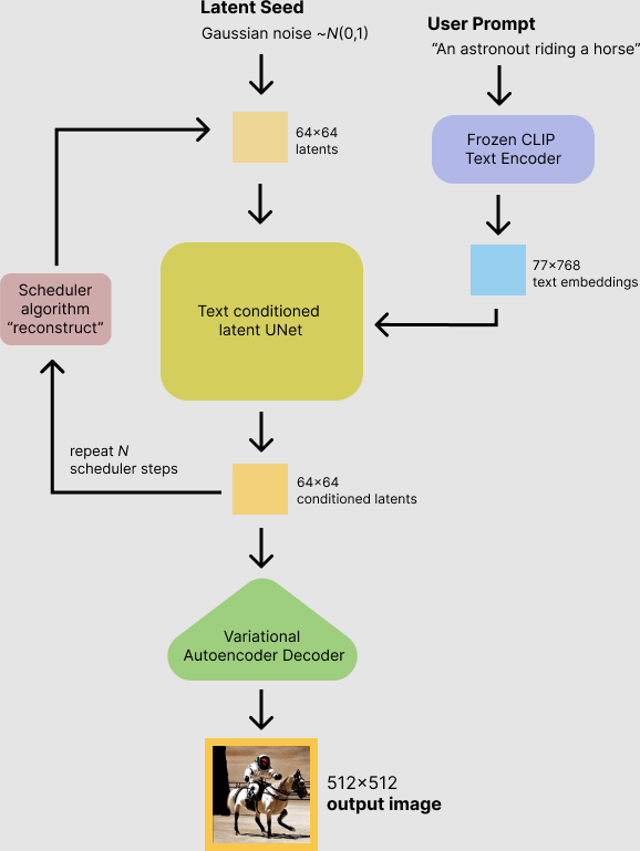
The stable diffusion model takes each a latent seed and a text prompt as an input. The latent seed is then used to generate random latent image representations of size $64\times 6464\; times\; 64$

Next the U-Net iteratively denoises the random latent image representations while being conditioned on the text embeddings. The output of the U-Net, being the noise residual, is used to compute a denoised latent image representation via a scheduler algorithm. Many various scheduler algorithms may be used for this computation, each having its pro- and cons. For Stable Diffusion, we recommend using one in every of:

Theory on how the scheduler algorithm function is out-of-scope for this notebook, but briefly one should keep in mind that they compute the anticipated denoised image representation from the previous noise representation and the anticipated noise residual.
For more information, we recommend looking into Elucidating the Design Space of Diffusion-Based Generative Models

The denoising process is repeated ca. 50 times to step-by-step retrieve higher latent image representations.
Once complete, the latent image representation is decoded by the decoder a part of the variational auto encoder.

After this transient introduction to Latent and Stable Diffusion, let’s have a look at tips on how to make advanced use of 🤗 Hugging Face diffusers library!

Writing your individual inference pipeline

Finally, we show how you possibly can create custom diffusion pipelines with diffusers.
Writing a custom inference pipeline is a sophisticated use of the diffusers library that may be useful to change out certain components, similar to the VAE or scheduler explained above.

For instance, we’ll show tips on how to use Stable Diffusion with a distinct scheduler, namely Katherine Crowson’s K-LMS scheduler added in this PR.

The pre-trained model includes all of the components required to setup a whole diffusion pipeline. They’re stored in the next folders:

• text_encoder: Stable Diffusion uses CLIP, but other diffusion models may use other encoders similar to BERT.
• tokenizer. It must match the one utilized by the text_encoder model.
• scheduler: The scheduling algorithm used to progressively add noise to the image during training.
• unet: The model used to generate the latent representation of the input.
• vae: Autoencoder module that we’ll use to decode latent representations into real images.

We are able to load the components by referring to the folder they were saved, using the subfolder argument to from_pretrained.

from transformers import CLIPTextModel, CLIPTokenizer
from diffusers import AutoencoderKL, UNet2DConditionModel, PNDMScheduler


vae = AutoencoderKL.from_pretrained("CompVis/stable-diffusion-v1-4", subfolder="vae")


tokenizer = CLIPTokenizer.from_pretrained("openai/clip-vit-large-patch14")
text_encoder = CLIPTextModel.from_pretrained("openai/clip-vit-large-patch14")


unet = UNet2DConditionModel.from_pretrained("CompVis/stable-diffusion-v1-4", subfolder="unet")

Now as a substitute of loading the pre-defined scheduler, we load the K-LMS scheduler with some fitting parameters.

from diffusers import LMSDiscreteScheduler

scheduler = LMSDiscreteScheduler(beta_start=0.00085, beta_end=0.012, beta_schedule="scaled_linear", num_train_timesteps=1000)

Next, let’s move the models to GPU.

torch_device = "cuda"
vae.to(torch_device)
text_encoder.to(torch_device)
unet.to(torch_device) 

We now define the parameters we’ll use to generate images.

Note that guidance_scale is defined analog to the guidance weight w of equation (2) within the Imagen paper. guidance_scale == 1 corresponds to doing no classifier-free guidance. Here we set it to 7.5 as also done previously.

In contrast to the previous examples, we set num_inference_steps to 100 to get an excellent more defined image.

prompt = ["a photograph of an astronaut riding a horse"]

height = 512                        
width = 512                         

num_inference_steps = 100           

guidance_scale = 7.5                

generator = torch.manual_seed(0)    

batch_size = len(prompt)

First, we get the text_embeddings for the passed prompt.
These embeddings will probably be used to condition the UNet model and guide the image generation towards something that ought to resemble the input prompt.

text_input = tokenizer(prompt, padding="max_length", max_length=tokenizer.model_max_length, truncation=True, return_tensors="pt")

text_embeddings = text_encoder(text_input.input_ids.to(torch_device))[0]

We’ll also get the unconditional text embeddings for classifier-free guidance, that are just the embeddings for the padding token (empty text). They should have the identical shape because the conditional text_embeddings (batch_size and seq_length)

max_length = text_input.input_ids.shape[-1]
uncond_input = tokenizer(
    [""] * batch_size, padding="max_length", max_length=max_length, return_tensors="pt"
)
uncond_embeddings = text_encoder(uncond_input.input_ids.to(torch_device))[0]   

For classifier-free guidance, we’d like to do two forward passes: one with the conditioned input (text_embeddings), and one other with the unconditional embeddings (uncond_embeddings). In practice, we are able to concatenate each right into a single batch to avoid doing two forward passes.

text_embeddings = torch.cat([uncond_embeddings, text_embeddings])

Next, we generate the initial random noise.

latents = torch.randn(
    (batch_size, unet.in_channels, height // 8, width // 8),
    generator=generator,
)
latents = latents.to(torch_device)

If we examine the latents at this stage we’ll see their shape is torch.Size([1, 4, 64, 64]), much smaller than the image we wish to generate. The model will transform this latent representation (pure noise) right into a 512 × 512 image afterward.

Next, we initialize the scheduler with our chosen num_inference_steps.
This may compute the sigmas and exact time step values for use in the course of the denoising process.

scheduler.set_timesteps(num_inference_steps)

The K-LMS scheduler must multiply the latents by its sigma values. Let’s do that here:

latents = latents * scheduler.init_noise_sigma

We’re ready to jot down the denoising loop.

from tqdm.auto import tqdm

scheduler.set_timesteps(num_inference_steps)

for t in tqdm(scheduler.timesteps):
    
    latent_model_input = torch.cat([latents] * 2)

    latent_model_input = scheduler.scale_model_input(latent_model_input, timestep=t)

    
    with torch.no_grad():
        noise_pred = unet(latent_model_input, t, encoder_hidden_states=text_embeddings).sample

    
    noise_pred_uncond, noise_pred_text = noise_pred.chunk(2)
    noise_pred = noise_pred_uncond + guidance_scale * (noise_pred_text - noise_pred_uncond)

    
    latents = scheduler.step(noise_pred, t, latents).prev_sample

We now use the vae to decode the generated latents back into the image.

latents = 1 / 0.18215 * latents
with torch.no_grad():
    image = vae.decode(latents).sample

And eventually, let’s convert the image to PIL so we are able to display or put it aside.

image = (image / 2 + 0.5).clamp(0, 1)
image = image.detach().cpu().permute(0, 2, 3, 1).numpy()
images = (image * 255).round().astype("uint8")
pil_images = [Image.fromarray(image) for image in images]
pil_images[0]

We have gone from the essential use of Stable Diffusion using 🤗 Hugging Face Diffusers to more advanced uses of the library, and we tried to introduce all of the pieces in a contemporary diffusion system. When you liked this topic and wish to learn more, we recommend the next resources:

Citation:

@article{patil2022stable,
  creator = {Patil, Suraj and Cuenca, Pedro and Lambert, Nathan and von Platen, Patrick},
  title = {Stable Diffusion with 🧨 Diffusers},
  journal = {Hugging Face Blog},
  yr = {2022},
  note = {[https://huggingface.co/blog/rlhf](https://huggingface.co/blog/stable_diffusion)},
}