Mixture of Experts Explained

With the discharge of Mixtral 8x7B (announcement, model card), a category of transformer has change into the most popular topic within the open AI community: Mixture of Experts, or MoEs for brief. On this blog post, we take a have a look at the constructing blocks of MoEs, how they’re trained, and the tradeoffs to think about when serving them for inference.

Let’s dive in!

Table of Contents

TL;DR

MoEs:

• Are pretrained much faster vs. dense models
• Have faster inference in comparison with a model with the identical variety of parameters
• Require high VRAM as all experts are loaded in memory
• Face many challenges in fine-tuning, but recent work with MoE instruction-tuning is promising

Let’s dive in!

What’s a Mixture of Experts (MoE)?

The dimensions of a model is some of the vital axes for higher model quality. Given a set computing budget, training a bigger model for fewer steps is best than training a smaller model for more steps.

Mixture of Experts enable models to be pretrained with far less compute, which implies you’ll be able to dramatically scale up the model or dataset size with the identical compute budget as a dense model. Specifically, a MoE model should achieve the identical quality as its dense counterpart much faster during pretraining.

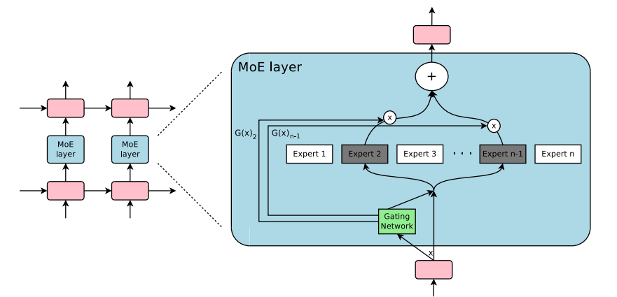
So, what exactly is a MoE? Within the context of transformer models, a MoE consists of two principal elements:

• Sparse MoE layers are used as a substitute of dense feed-forward network (FFN) layers. MoE layers have a certain variety of “experts” (e.g. 8), where each expert is a neural network. In practice, the experts are FFNs, but they can be more complex networks or perhaps a MoE itself, resulting in hierarchical MoEs!
• A gate network or router, that determines which tokens are sent to which expert. For instance, within the image below, the token “More” is shipped to the second expert, and the token “Parameters” is shipped to the primary network. As we’ll explore later, we will send a token to a couple of expert. How you can route a token to an authority is certainly one of the massive decisions when working with MoEs – the router consists of learned parameters and is pretrained similtaneously the remainder of the network.

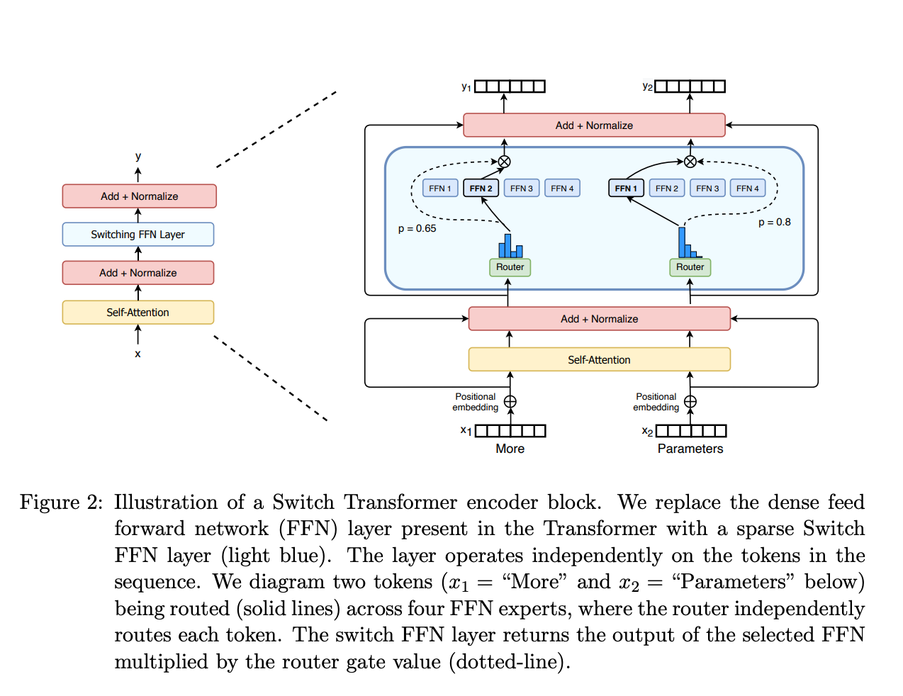
So, to recap, in MoEs we replace every FFN layer of the transformer model with an MoE layer, which consists of a gate network and a certain variety of experts.

Although MoEs provide advantages like efficient pretraining and faster inference in comparison with dense models, additionally they include challenges:

• Training: MoEs enable significantly more compute-efficient pretraining, but they’ve historically struggled to generalize during fine-tuning, resulting in overfitting.
• Inference: Although a MoE might need many parameters, just some of them are used during inference. This results in much faster inference in comparison with a dense model with the identical variety of parameters. Nonetheless, all parameters should be loaded in RAM, so memory requirements are high. For instance, given a MoE like Mixtral 8x7B, we’ll have to have enough VRAM to carry a dense 47B parameter model. Why 47B parameters and never 8 x 7B = 56B? That’s because in MoE models, only the FFN layers are treated as individual experts, and the remainder of the model parameters are shared. At the identical time, assuming just two experts are getting used per token, the inference speed (FLOPs) is like using a 12B model (versus a 14B model), since it computes 2x7B matrix multiplications, but with some layers shared (more on this soon).

Now that we now have a rough idea of what a MoE is, let’s take a have a look at the research developments that led to their invention.

A Transient History of MoEs

The roots of MoEs come from the 1991 paper Adaptive Mixture of Local Experts. The thought, akin to ensemble methods, was to have a supervised procedure for a system composed of separate networks, each handling a special subset of the training cases. Each separate network, or expert, focuses on a special region of the input space. How is the expert chosen? A gating network determines the weights for every expert. During training, each the expert and the gating are trained.

Between 2010-2015, two different research areas contributed to later MoE advancement:

• Experts as components: In the normal MoE setup, the entire system comprises a gating network and multiple experts. MoEs as the entire model have been explored in SVMs, Gaussian Processes, and other methods. The work by Eigen, Ranzato, and Ilya explored MoEs as components of deeper networks. This permits having MoEs as layers in a multilayer network, making it possible for the model to be each large and efficient concurrently.
• Conditional Computation: Traditional networks process all input data through every layer. In this era, Yoshua Bengio researched approaches to dynamically activate or deactivate components based on the input token.

These works led to exploring a mix of experts within the context of NLP. Concretely, Shazeer et al. (2017, with “et al.” including Geoffrey Hinton and Jeff Dean, Google’s Chuck Norris) scaled this concept to a 137B LSTM (the de-facto NLP architecture back then, created by Schmidhuber) by introducing sparsity, allowing to maintain very fast inference even at high scale. This work focused on translation but faced many challenges, corresponding to high communication costs and training instabilities.

MoEs have allowed training multi-trillion parameter models, corresponding to the open-sourced 1.6T parameters Switch Transformers, amongst others. MoEs have also been explored in Computer Vision, but this blog post will give attention to the NLP domain.

What’s Sparsity?

Sparsity uses the thought of conditional computation. While in dense models all of the parameters are used for all of the inputs, sparsity allows us to only run some parts of the entire system.

Let’s dive deeper into Shazeer’s exploration of MoEs for translation. The thought of conditional computation (parts of the network are lively on a per-example basis) allows one to scale the scale of the model without increasing the computation, and hence, this led to 1000’s of experts getting used in each MoE layer.

This setup introduces some challenges. For instance, although large batch sizes are often higher for performance, batch sizes in MOEs are effectively reduced as data flows through the lively experts. For instance, if our batched input consists of 10 tokens, five tokens might end in a single expert, and the opposite five tokens might end in five different experts, resulting in uneven batch sizes and underutilization. The Making MoEs go brrr section below will discuss other challenges and solutions.

How can we solve this? A learned gating network (G) decides which experts (E) to send an element of the input:

$$y=\sum _{i=1}^{n}G(x{)}_i{E}_i(x)y\; =\; sum\_\{i=1\}^\{n\}\; G(x)\_i\; E\_i(x)$$

On this setup, all experts are run for all inputs – it’s a weighted multiplication. But, what happens if G is 0? If that’s the case, there’s no have to compute the respective expert operations and hence we save compute. What’s a typical gating function? In essentially the most traditional setup, we just use a straightforward network with a softmax function. The network will learn which expert to send the input.

$$G_{\sigma }(x)=\text{Softmax}(x\cdot W_g)G\_sigma(x)\; =\; text\{Softmax\}(x\; cdot\; W\_g)$$

Shazeer’s work also explored other gating mechanisms, corresponding to Noisy Top-k Gating. This gating approach introduces some (tunable) noise after which keeps the highest k values. That’s:

1. We add some noise

$$H(x{)}_i=(x\cdot W_{\text{g}}{)}_i+\text{StandardNormal()}\cdot \text{Softplus}((x\cdot W_{\text{noise}}{)}_i)H(x)\_i\; =\; (x\; cdot\; W\_\{text\{g\}\})\_i\; +\; text\{StandardNormal()\}\; cdot\; text\{Softplus\}((x\; cdot\; W\_\{text\{noise\}\})\_i)$$

H(x)i​=(x⋅Wg​)i​+StandardNormal()⋅Softplus((x⋅Wnoise​)i​)

2. We only pick the highest k

3. We apply the softmax.

$$G(x)=\text{Softmax}(\text{KeepTopK}(H(x),k))G(x)\; =\; text\{Softmax\}(text\{KeepTopK\}(H(x),\; k))$$

This sparsity introduces some interesting properties. By utilizing a low enough k (e.g. one or two), we will train and run inference much faster than if many experts were activated. Why not only select the highest expert? The initial conjecture was that routing to a couple of expert was needed to have the gate learn how you can path to different experts, so not less than two experts needed to be picked. The Switch Transformers section revisits this decision.

Why will we add noise? That’s for load balancing!

Load balancing tokens for MoEs

As discussed before, if all our tokens are sent to simply a couple of popular experts, that can make training inefficient. In a traditional MoE training, the gating network converges to mostly activate the identical few experts. This self-reinforces as favored experts are trained quicker and hence chosen more. To mitigate this, an auxiliary loss is added to encourage giving all experts equal importance. This loss ensures that each one experts receive a roughly equal number of coaching examples. The next sections will even explore the concept of expert capability, which introduces a threshold of what number of tokens may be processed by an authority. In transformers, the auxiliary loss is exposed via the aux_loss parameter.

MoEs and Transformers

Transformers are a really clear case that scaling up the variety of parameters improves the performance, so it’s not surprising that Google explored this with GShard, which explores scaling up transformers beyond 600 billion parameters.

GShard replaces every other FFN layer with an MoE layer using top-2 gating in each the encoder and the decoder. The following image shows how this looks like for the encoder part. This setup is kind of useful for large-scale computing: once we scale to multiple devices, the MoE layer is shared across devices while all the opposite layers are replicated. That is further discussed within the “Making MoEs go brrr” section.

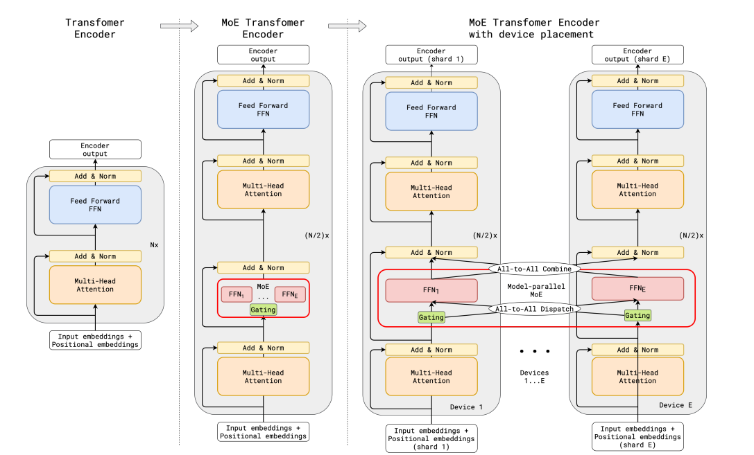
To keep up a balanced load and efficiency at scale, the GShard authors introduced a few changes along with an auxiliary loss much like the one discussed within the previous section:

• Random routing: in a top-2 setup, we all the time pick the highest expert, however the second expert is picked with probability proportional to its weight.
• Expert capability: we will set a threshold of what number of tokens may be processed by one expert. If each experts are at capability, the token is taken into account overflowed, and it’s sent to the following layer via residual connections (or dropped entirely in other projects). This idea will change into some of the vital concepts for MoEs. Why is expert capability needed? Since all tensor shapes are statically determined at compilation time, but we cannot know the way many tokens will go to every expert ahead of time, we’d like to repair the capability factor.

The GShard paper has contributions by expressing parallel computation patterns that work well for MoEs, but discussing that’s outside the scope of this blog post.

Note: once we run inference, just some experts shall be triggered. At the identical time, there are shared computations, corresponding to self-attention, which is applied for all tokens. That’s why once we talk of a 47B model of 8 experts, we will run with the compute of a 12B dense model. If we use top-2, 14B parameters could be used. But on condition that the eye operations are shared (amongst others), the actual variety of used parameters is 12B.

Switch Transformers

Although MoEs showed plenty of promise, they struggle with training and fine-tuning instabilities. Switch Transformers is a really exciting work that deep dives into these topics. The authors even released a 1.6 trillion parameters MoE on Hugging Face with 2048 experts, which you’ll run with transformers. Switch Transformers achieved a 4x pre-train speed-up over T5-XXL.

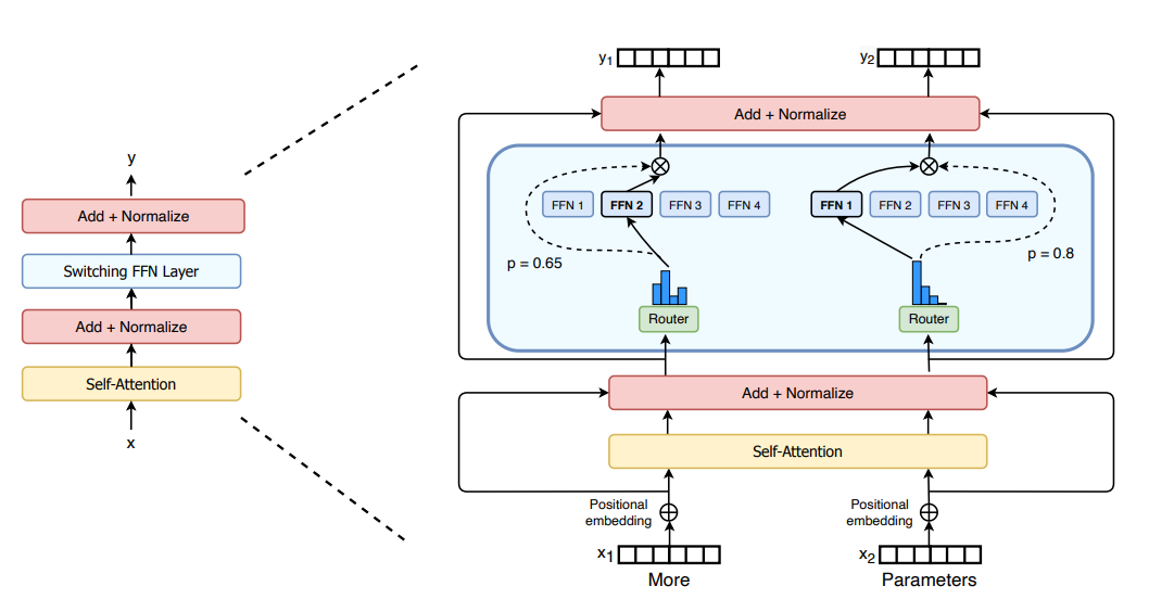
Just as in GShard, the authors replaced the FFN layers with a MoE layer. The Switch Transformers paper proposes a Switch Transformer layer that receives two inputs (two different tokens) and has 4 experts.

Contrary to the initial idea of using not less than two experts, Switch Transformers uses a simplified single-expert strategy. The results of this approach are:

• The router computation is reduced
• The batch size of every expert may be not less than halved
• Communication costs are reduced
• Quality is preserved

Switch Transformers also explores the concept of expert capability.

$$\text{Expert Capability}=\left(\frac{\text{tokens per batch}}{\text{number of experts}}\right)\times \text{capability factor}text\{Expert\; Capability\}\; =\; left(frac\{text\{tokens\; per\; batch\}\}\{text\{variety\; of\; experts\}\}right)\; times\; text\{capability\; factor\}$$

Expert Capability=(number of expertstokens per batch​)×capability factor

The capability suggested above evenly divides the variety of tokens within the batch across the variety of experts. If we use a capability factor greater than 1, we offer a buffer for when tokens usually are not perfectly balanced. Increasing the capability will result in dearer inter-device communication, so it’s a trade-off to be mindful. Specifically, Switch Transformers perform well at low capability aspects (1-1.25)

Switch Transformer authors also revisit and simplify the load balancing loss mentioned within the sections. For every Switch layer, the auxiliary loss is added to the overall model loss during training. This loss encourages uniform routing and may be weighted using a hyperparameter.

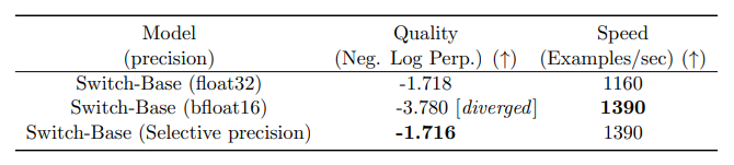
The authors also experiment with selective precision, corresponding to training the experts with bfloat16 while using full precision for the remainder of the computations. Lower precision reduces communication costs between processors, computation costs, and memory for storing tensors. The initial experiments, by which each the experts and the gate networks were trained in bfloat16, yielded more unstable training. This was, specifically, as a result of the router computation: because the router has an exponentiation function, having higher precision is very important. To mitigate the instabilities, full precision was used for the routing as well.

This notebook showcases fine-tuning Switch Transformers for summarization, but we recommend first reviewing the fine-tuning section.

Switch Transformers uses an encoder-decoder setup by which they did a MoE counterpart of T5. The GLaM paper explores pushing up the size of those models by training a model matching GPT-3 quality using 1/3 of the energy (yes, because of the lower amount of computing needed to coach a MoE, they will reduce the carbon footprint by as much as an order of magnitude). The authors focused on decoder-only models and few-shot and one-shot evaluation somewhat than fine-tuning. They used Top-2 routing and far larger capability aspects. As well as, they explored the capability factor as a metric one can change during training and evaluation depending on how much computing one wants to make use of.

Stabilizing training with router Z-loss

The balancing loss previously discussed can result in instability issues. We are able to use many methods to stabilize sparse models on the expense of quality. For instance, introducing dropout improves stability but results in lack of model quality. Alternatively, adding more multiplicative components improves quality but decreases stability.

Router z-loss, introduced in ST-MoE, significantly improves training stability without quality degradation by penalizing large logits entering the gating network. Since this loss encourages absolute magnitude of values to be smaller, roundoff errors are reduced, which may be quite impactful for exponential functions corresponding to the gating. We recommend reviewing the paper for details.

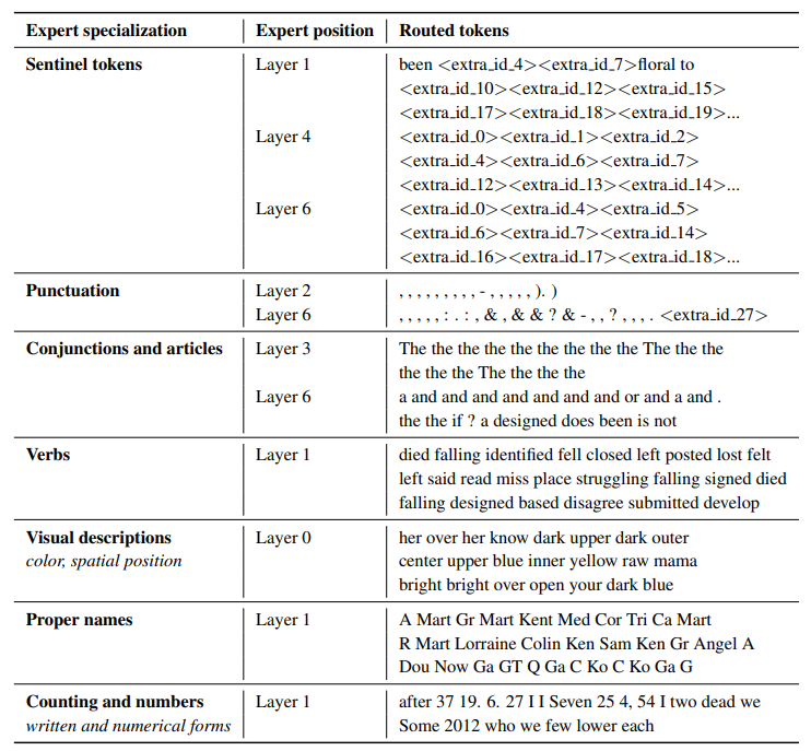
What does an authority learn?

The ST-MoE authors observed that encoder experts concentrate on a gaggle of tokens or shallow concepts. For instance, we’d end with a punctuation expert, a correct noun expert, etc. Alternatively, the decoder experts have less specialization. The authors also trained in a multilingual setup. Although one could imagine each expert specializing in a language, the other happens: as a result of token routing and cargo balancing, there isn’t any single expert specialized in any given language.

How does scaling the variety of experts impact pretraining?

More experts result in improved sample efficiency and faster speedup, but these are diminishing gains (especially after 256 or 512), and more VRAM shall be needed for inference. The properties studied in Switch Transformers at large scale were consistent at small scale, even with 2, 4, or 8 experts per layer.

Fantastic-tuning MoEs

Mixtral is supported with version 4.36.0 of transformers. You possibly can install it with pip install transformers==4.36.0 --upgrade

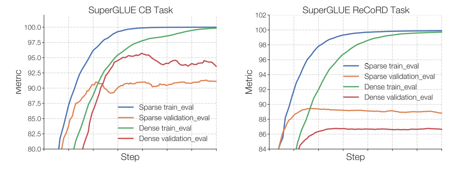
The overfitting dynamics are very different between dense and sparse models. Sparse models are more liable to overfitting, so we will explore higher regularization (e.g. dropout) throughout the experts themselves (e.g. we will have one dropout rate for the dense layers and one other, higher, dropout for the sparse layers).

One query is whether or not to make use of the auxiliary loss for fine-tuning. The ST-MoE authors experimented with turning off the auxiliary loss, and the standard was not significantly impacted, even when as much as 11% of the tokens were dropped. Token dropping may be a type of regularization that helps prevent overfitting.

Switch Transformers observed that at a set pretrain perplexity, the sparse model does worse than the dense counterpart in downstream tasks, especially on reasoning-heavy tasks corresponding to SuperGLUE. Alternatively, for knowledge-heavy tasks corresponding to TriviaQA, the sparse model performs disproportionately well. The authors also observed that a fewer variety of experts helped at fine-tuning. One other statement that confirmed the generalization issue is that the model did worse in smaller tasks but did well in larger tasks.

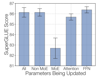
One could experiment with freezing all non-expert weights. That’s, we’ll only update the MoE layers. This results in an enormous performance drop. We could try the other: freezing only the parameters in MoE layers, which worked almost in addition to updating all parameters. This may also help speed up and reduce memory for fine-tuning. This may be somewhat counter-intuitive as 80% of the parameters are within the MoE layers (within the ST-MoE project). Their hypothesis for that architecture is that, as expert layers only occur every 1/4 layers, and every token sees at most two experts per layer, updating the MoE parameters affects much fewer layers than updating other parameters.

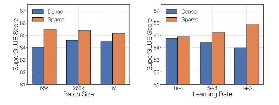
One last part to think about when fine-tuning sparse MoEs is that they’ve different fine-tuning hyperparameter setups – e.g., sparse models are likely to profit more from smaller batch sizes and better learning rates.

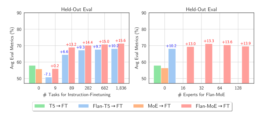
At this point, you may be a bit sad that individuals have struggled to fine-tune MoEs. Excitingly, a recent paper, MoEs Meets Instruction Tuning (July 2023), performs experiments doing:

• Single task fine-tuning
• Multi-task instruction-tuning
• Multi-task instruction-tuning followed by single-task fine-tuning

When the authors fine-tuned the MoE and the T5 equivalent, the T5 equivalent was higher. When the authors fine-tuned the Flan T5 (T5 instruct equivalent) MoE, the MoE performed significantly higher. Not only this, the development of the Flan-MoE over the MoE was larger than Flan T5 over T5, indicating that MoEs might profit rather more from instruction tuning than dense models. MoEs profit more from a better variety of tasks. Unlike the previous discussion suggesting to show off the auxiliary loss function, the loss actually prevents overfitting.

When to make use of sparse MoEs vs dense models?

Experts are useful for top throughput scenarios with many machines. Given a set compute budget for pretraining, a sparse model shall be more optimal. For low throughput scenarios with little VRAM, a dense model shall be higher.

Note: one cannot directly compare the variety of parameters between sparse and dense models, as each represent significantly various things.

Making MoEs go brrr

The initial MoE work presented MoE layers as a branching setup, resulting in slow computation as GPUs usually are not designed for it and resulting in network bandwidth becoming a bottleneck because the devices have to send info to others. This section will discuss some existing work to make pretraining and inference with these models more practical. MoEs go brrrrr.

Parallelism

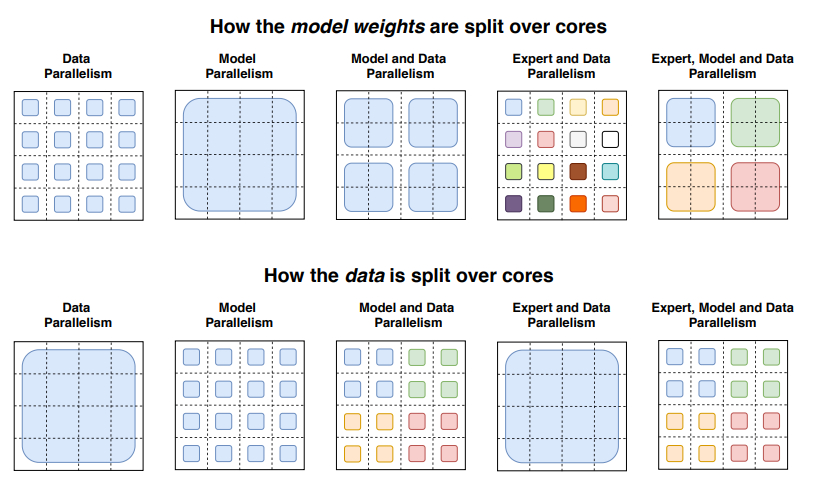
Let’s do a transient review of parallelism:

• Data parallelism: the identical weights are replicated across all cores, and the information is partitioned across cores.
• Model parallelism: the model is partitioned across cores, and the information is replicated across cores.
• Model and data parallelism: we will partition the model and the information across cores. Note that different cores process different batches of information.
• Expert parallelism: experts are placed on different employees. If combined with data parallelism, each core has a special expert and the information is partitioned across all cores

With expert parallelism, experts are placed on different employees, and every employee takes a special batch of coaching samples. For non-MoE layers, expert parallelism behaves the identical as data parallelism. For MoE layers, tokens within the sequence are sent to employees where the specified experts reside.

Capability Factor and communication costs

Increasing the capability factor (CF) increases the standard but increases communication costs and memory of activations. If all-to-all communications are slow, using a smaller capability factor is best. An excellent place to begin is using top-2 routing with 1.25 capability factor and having one expert per core. During evaluation, the capability factor may be modified to scale back compute.

Serving techniques

You possibly can deploy mistralai/Mixtral-8x7B-Instruct-v0.1 to Inference Endpoints.

A giant downside of MoEs is the big variety of parameters. For local use cases, one might need to use a smaller model. Let’s quickly discuss a couple of techniques that may also help with serving:

• The Switch Transformers authors did early distillation experiments. By distilling a MoE back to its dense counterpart, they may keep 30-40% of the sparsity gains. Distillation, hence, provides the advantages of faster pretraining and using a smaller model in production.
• Recent approaches modify the routing to route full sentences or tasks to an authority, permitting extracting sub-networks for serving.
• Aggregation of Experts (MoE): this system merges the weights of the experts, hence reducing the variety of parameters at inference time.

More on efficient training

FasterMoE (March 2022) analyzes the performance of MoEs in highly efficient distributed systems and analyzes the theoretical limit of various parallelism strategies, in addition to techniques to skew expert popularity, fine-grained schedules of communication that reduce latency, and an adjusted topology-aware gate that picks experts based on the bottom latency, resulting in a 17x speedup.

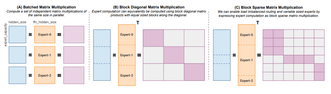
Megablocks (Nov 2022) explores efficient sparse pretraining by providing latest GPU kernels that may handle the dynamism present in MoEs. Their proposal never drops tokens and maps efficiently to modern hardware, resulting in significant speedups. What’s the trick? Traditional MoEs use batched matrix multiplication, which assumes all experts have the identical shape and the identical variety of tokens. In contrast, Megablocks expresses MoE layers as block-sparse operations that may accommodate imbalanced task.

Open Source MoEs

There are nowadays several open source projects to coach MoEs:

Within the realm of released open access MoEs, you’ll be able to check:

Exciting directions of labor

Further experiments on distilling a sparse MoE back to a dense model with fewer parameters but similar quality.

One other area shall be quantization of MoEs. QMoE (Oct. 2023) is an excellent step on this direction by quantizing the MoEs to lower than 1 bit per parameter, hence compressing the 1.6T Switch Transformer which uses 3.2TB accelerator to simply 160GB.

So, TL;DR, some interesting areas to explore:

• Distilling Mixtral right into a dense model
• Explore model merging techniques of the experts and their impact in inference time
• Perform extreme quantization techniques of Mixtral

Some resources

Citation

@misc {sanseviero2023moe,
    writer       = { Omar Sanseviero and
                     Lewis Tunstall and
                     Philipp Schmid and
                     Sourab Mangrulkar and
                     Younes Belkada and
                     Pedro Cuenca
                   },
    title        = { Mixture of Experts Explained },
    12 months         = 2023,
    url          = { https://huggingface.co/blog/moe },
    publisher    = { Hugging Face Blog }
}

Sanseviero, et al., "Mixture of Experts Explained", Hugging Face Blog, 2023.