lower your expenses, time and carbon with open source

Must you fine-tune your personal model or use an LLM API? Creating your personal model puts you in full control but requires expertise in data collection, training, and deployment. LLM APIs are much easier to make use of but force you to send your data to a 3rd party and create costly dependencies on LLM providers. This blog post shows how you’ll be able to mix the convenience of LLMs with the control and efficiency of customized models.

In a case study on identifying investor sentiment within the news, we show use an open-source LLM to create synthetic data to coach your customized model in a couple of steps. Our resulting custom RoBERTa model can analyze a big news corpus for around $2.7 in comparison with $3061 with GPT4; emits around 0.12 kg CO2 in comparison with very roughly 735 to 1100 kg CO2 with GPT4; with a latency of 0.13 seconds in comparison with often multiple seconds with GPT4; while acting on par with GPT4 at identifying investor sentiment (each 94% accuracy and 0.94 F1 macro). We offer reusable notebooks, which you’ll apply to your personal use cases.

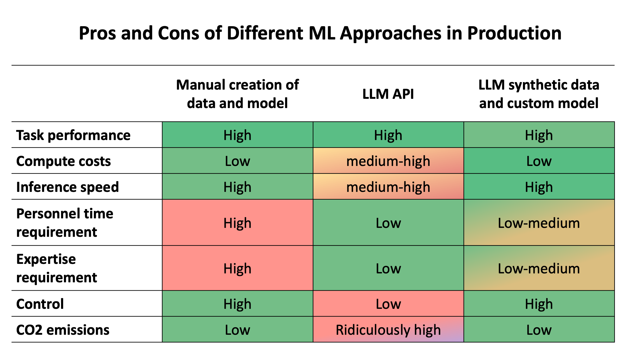
Table of Contents

1. The issue: There isn’t a data on your use-case

Imagine your boss asking you to construct a sentiment evaluation system on your company. You can see 100,000+ datasets on the Hugging Face Hub, 450~ of which have the word “sentiment” within the title, covering sentiment on Twitter, in poems, or in Hebrew. That is great, but when, for instance, you’re employed in a financial institution and you have to track sentiment towards the particular brands in your portfolio, none of those datasets are useful on your task. With the hundreds of thousands of tasks firms could tackle with machine learning, it’s unlikely that somebody already collected and published data on the precise use case your organization is trying to unravel.

Given this lack of task-specific datasets and models, many individuals turn to general-purpose LLMs. These models are so large and general that they’ll tackle most tasks out of the box with impressive accuracy. Their easy-to-use APIs eliminate the necessity for expertise in fine-tuning and deployment. Their foremost disadvantages are size and control: with tons of of billions or trillions of parameters, these models are inefficient and only run on compute clusters controlled by a couple of firms.

2. The answer: Synthetic data to show efficient students

In 2023, one development fundamentally modified the machine-learning landscape: LLMs began reaching parity with human data annotators. There’s now ample evidence showing that one of the best LLMs outperform crowd employees and are reaching parity with experts in creating quality (synthetic) data (e.g. Zheng et al. 2023, Gilardi et al. 2023, He et al. 2023). It is tough to overstate the importance of this development. The important thing bottleneck for creating tailored models was the cash, time, and expertise required to recruit and coordinate human employees to create tailored training data. With LLMs starting to succeed in human parity, high-quality annotation labor is now available through APIs; reproducible annotation instructions may be sent as prompts; and artificial data is returned almost instantaneously with compute because the only bottleneck.

In 2024, this approach will turn out to be commercially viable and boost the worth of open-source for small and enormous businesses. For many of 2023, industrial use of LLMs for annotation labor was blocked as a result of restrictive business terms by LLM API providers. With models like Mixtral-8x7B-Instruct-v0.1 by Mistral, LLM annotation labor and artificial data now turn out to be open for industrial use. Mixtral performs on par with GPT3.5, and due to its Apache 2.0 license, its synthetic data outputs may be used as training data for smaller, specialized models (the “students”) for industrial use-cases. This blog post provides an example of how it will significantly speed up the creation of your personal tailored models while drastically reducing long-term inference costs.

3. Case study: Monitoring financial sentiment

Imagine you might be a developer in a big investment firm tasked with monitoring economic news sentiment toward firms in your investment portfolio. Until recently, you had two foremost options:

1. You might fine-tune your personal model. This requires writing annotation instructions, creating an annotation interface, recruiting (crowd) employees, introducing quality assurance measures to handle low-quality data, fine-tuning a model on this data, and deploying it.

2. Or you can send your data with instructions to an LLM API. You skip fine-tuning and deployment entirely, and also you reduce the information evaluation process to writing instructions (prompts), which you send to an “LLM annotator” behind an API. On this case, the LLM API is your final inference solution and you employ the LLM’s outputs directly on your evaluation.

Although Option 2 is dearer at inference time and requires you to send sensitive data to a 3rd party, it’s significantly easier to establish than Option 1 and, due to this fact, utilized by many developers.

In 2024, synthetic data provides a 3rd option: combining the fee advantages of Option 1 with the ease-of-use of Option 2. Simply put, you should use an LLM (the “teacher”) to annotate a small sample of knowledge for you, and you then fine-tune a smaller, more efficient LM (the “student”) on this data. This approach may be implemented in a couple of easy steps.

3.1 Prompt an LLM to annotate your data

We use the financial_phrasebank sentiment dataset as a running example, but you’ll be able to adapt the code for another use case. The financial_phrasebank task is a 3-class classification task, where 16 experts annotated sentences from financial news on Finnish firms as “positive” / “negative” / “neutral” from an investor perspective (Malo et al. 2013). For instance, the dataset incorporates the sentence “For the last quarter of 2010, Componenta’s net sales doubled to EUR131m from EUR76m for a similar period a yr earlier”, which was categorized as “positive” from an investor perspective by annotators.

We start by installing a couple of required libraries.

!pip install datasets  
!pip install huggingface_hub  
!pip install requests  
!pip install scikit-learn  
!pip install pandas  
!pip install tqdm  

We will then download the instance dataset with its expert annotations.

from datasets import load_dataset

dataset = load_dataset("financial_phrasebank", "sentences_allagree", split='train')


label_map = {
    i: label_text 
    for i, label_text in enumerate(dataset.features["label"].names)
}

def add_label_text(example):
    example["label_text"] = label_map[example["label"]]
    return example

dataset = dataset.map(add_label_text)

print(dataset)

Now we write a brief annotation instruction tailored to the financial_phrasebank task and format it as an LLM prompt. This prompt is analogous to the instructions you normally provide to crowd employees.

prompt_financial_sentiment = """
You're a highly qualified expert trained to annotate machine learning training data.

Your task is to research the sentiment within the TEXT below from an investor perspective and label it with just one the three labels:
positive, negative, or neutral.

Base your label decision only on the TEXT and don't speculate e.g. based on prior knowledge about an organization. 

Don't provide any explanations and only respond with considered one of the labels as one word: negative, positive, or neutral

Examples:
Text: Operating profit increased, from EUR 7m to 9m in comparison with the previous reporting period.
Label: positive
Text: The corporate generated net sales of 11.3 million euro this yr.
Label: neutral
Text: Profit before taxes decreased to EUR 14m, in comparison with EUR 19m within the previous period.	
Label: negative

Your TEXT to analyse:
TEXT: {text}
Label: """

Before we will pass this prompt to the API, we’d like so as to add some formatting to the prompt. Most LLMs today are fine-tuned with a particular chat template. This template consists of special tokens, which enable LLMs to tell apart between the user’s instructions, the system prompt, and its own responses in a chat history. Although we usually are not using the model as a chat bot here, omitting the chat template can still result in silently performance degradation. You should use the tokenizer so as to add the special tokens of the model’s chat template mechanically (read more here). For our example, we use the Mixtral-8x7B-Instruct-v0.1 model.

from transformers import AutoTokenizer

tokenizer = AutoTokenizer.from_pretrained("mistralai/Mixtral-8x7B-Instruct-v0.1")

chat_financial_sentiment = [{"role": "user", "content": prompt_financial_sentiment}]

prompt_financial_sentiment = tokenizer.apply_chat_template(chat_financial_sentiment, tokenize=False)

The formatted annotation instruction (prompt) can now be passed to the LLM API. We use the free Hugging Face serverless Inference API. The API is good for testing popular models. Note that you simply might encounter rate limits when you send an excessive amount of data to the free API, because it is shared amongst many users. For larger workloads, we recommend making a dedicated Inference Endpoint. A dedicated Inference Endpoint is actually your personal personal paid API, which you’ll flexibly activate and off.

We login with the huggingface_hub library to simply and safely handle our API token. Alternatively, you too can define your token as an environment variable (see the documentation).

import huggingface_hub
huggingface_hub.login()

We then define a straightforward generate_text function for sending our prompt and data to the API.

import os
import requests



API_URL = "https://api-inference.huggingface.co/models/mistralai/Mixtral-8x7B-Instruct-v0.1"


generation_params = dict(
    top_p=0.90,
    temperature=0.8,
    max_new_tokens=128,
    return_full_text=False,
    use_cache=False
)

def generate_text(prompt=None, generation_params=None):
    payload = {
        "inputs": prompt, 
        "parameters": {**generation_params}
    }
    response = requests.post(
        API_URL, 
        headers={"Authorization": f"Bearer {huggingface_hub.get_token()}"}, 
        json=payload
    )
    return response.json()[0]["generated_text"]

Because the LLM won’t at all times return the labels in the exact same harmonized format, we also define a brief clean_output function, which maps the string output from the LLM to our three possible labels.

labels = ["positive", "negative", "neutral"]

def clean_output(string, random_choice=True):
    for category in labels:
        if category.lower() in string.lower():
            return category
    
    if random_choice:
        return random.selection(labels)
    else:
        return "FAIL"

We will now send our texts to the LLM for annotation. The code below sends each text to the LLM API and maps the text output to our three clean categories. Note: iterating over each text and sending them to an API individually is inefficient in practice. APIs can process multiple texts concurrently, and you’ll be able to significantly speed up your API calls by sending batches of text to the API asynchronously. Yow will discover optimized code within the reproduction repository of this blog post.

output_simple = []
for text in dataset["sentence"]:
    
    prompt_formatted = prompt_financial_sentiment.format(text=text)
    
    output = generate_text(
        prompt=prompt_formatted, generation_params=generation_params
    )
    
    output_cl = clean_output(output, random_choice=True)
    output_simple.append(output_cl)

Based on this output, we will now calculate metrics to see how accurately the model did the duty without being trained on it.

from sklearn.metrics import classification_report

def compute_metrics(label_experts, label_pred):
    
    metrics_report = classification_report(
        label_experts, label_pred, digits=2, output_dict=True, zero_division='warn'
    )
    return metrics_report

label_experts = dataset["label_text"]
label_pred = output_simple

metrics = compute_metrics(label_experts, label_pred)

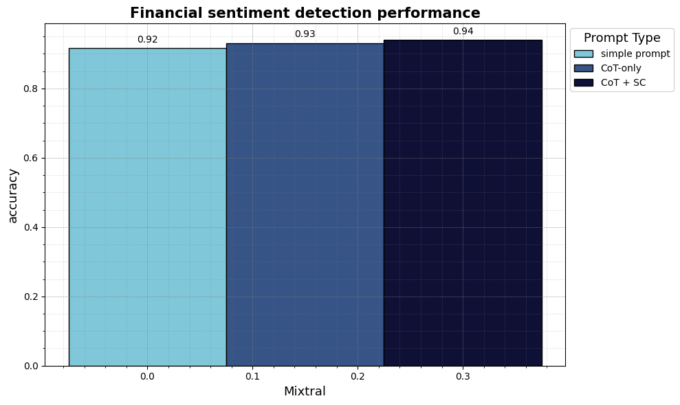
Based on the straightforward prompt, the LLM appropriately classified 91.6% of texts (0.916 accuracy and 0.916 F1 macro). That’s pretty good, on condition that it was not trained to do that specific task.

We will further improve this by utilizing two easy prompting techniques: Chain-of-Thought (CoT) and Self-Consistency (SC). CoT asks the model to first reason in regards to the correct label after which take the labeling decision as an alternative of immediately deciding on the right label. SC means sending the identical prompt with the identical text to the identical LLM multiple times. SC effectively gives the LLM multiple attempts per text with different reasoning paths, and if the LLM then responds “positive” twice and “neutral” once, we decide the bulk (”positive”) as the right label. Here is our updated prompt for CoT and SC:

prompt_financial_sentiment_cot = """
You're a highly qualified expert trained to annotate machine learning training data.

Your task is to briefly analyze the sentiment within the TEXT below from an investor perspective after which label it with just one the three labels:
positive, negative, neutral.

Base your label decision only on the TEXT and don't speculate e.g. based on prior knowledge about an organization. 

You first reason step-by-step in regards to the correct label after which return your label.

You ALWAYS respond only in the next JSON format: {{"reason": "...", "label": "..."}}
You simply respond with one single JSON response. 

Examples:
Text: Operating profit increased, from EUR 7m to 9m in comparison with the previous reporting period.
JSON response: {{"reason": "A rise in operating profit is positive for investors", "label": "positive"}}
Text: The corporate generated net sales of 11.3 million euro this yr.
JSON response: {{"reason": "The text only mentions financials without indication in the event that they are higher or worse than before", "label": "neutral"}}
Text: Profit before taxes decreased to EUR 14m, in comparison with EUR 19m within the previous period.	
JSON response: {{"reason": "A decrease in profit is negative for investors", "label": "negative"}}

Your TEXT to analyse:
TEXT: {text}
JSON response: """


chat_financial_sentiment_cot = [{"role": "user", "content": prompt_financial_sentiment_cot}]
prompt_financial_sentiment_cot = tokenizer.apply_chat_template(chat_financial_sentiment_cot, tokenize=False)

This can be a JSON prompt where we ask the LLM to return a structured JSON string with its “reason” as one key and the “label” as one other key. The foremost advantage of JSON is that we will parse it to a Python dictionary after which extract the “label”. We also can extract the “reason” if we wish to grasp the reasoning why the LLM selected this label.

The process_output_cot function parses the JSON string returned by the LLM and, in case the LLM doesn’t return valid JSON, it tries to discover the label with a straightforward string match from our clean_output function defined above.

import ast 

def process_output_cot(output):
    try: 
        output_dic = ast.literal_eval(output) 
        return output_dic
    except Exception as e:
        
        print(f"Parsing failed for output: {output}, Error: {e}")
        output_cl = clean_output(output, random_choice=False)
        output_dic = {"reason": "FAIL", "label": output_cl}
        return output_dic

We will now reuse our generate_text function from above with the brand new prompt, process the JSON Chain-of-Thought output with process_output_cot and send each prompt multiple times for Self-Consistency.

self_consistency_iterations = 3

output_cot_multiple = []
for _ in range(self_consistency_iterations):
    output_lst_step = []
    for text in tqdm(dataset["sentence"]):
        prompt_formatted = prompt_financial_sentiment_cot.format(text=text)
        output = generate_text(
            prompt=prompt_formatted, generation_params=generation_params
        )
        output_dic = process_output_cot(output)
        output_lst_step.append(output_dic["label"])

    output_cot_multiple.append(output_lst_step)

For every text, we now have three attempts by our LLM annotator to discover the right label with three different reasoning paths. The code below selects the bulk label from the three paths.

import pandas as pd
from collections import Counter

def find_majority(row):
    
    count = Counter(row)
    
    majority = count.most_common(1)[0]
    
    if majority[1] > 1:
        return majority[0]
    else: 
        return random.selection(labels)

df_output = pd.DataFrame(data=output_cot_multiple).T

df_output['label_pred_cot_multiple'] = df_output.apply(find_majority, axis=1)

Now, we will compare our improved LLM labels with the expert labels again and calculate metrics.

label_experts = dataset["label_text"]
label_pred_cot_multiple = df_output['label_pred_cot_multiple']

metrics_cot_multiple = compute_metrics(label_experts, label_pred_cot_multiple)

CoT and SC increased performance to 94.0% accuracy and 0.94 F1 macro. We’ve got improved performance by giving the model time to take into consideration its label decision and giving it multiple attempts. Note that CoT and SC cost additional compute. We’re essentially buying annotation accuracy with compute.

We’ve got now created an artificial training dataset due to these easy LLM API calls. We’ve got labeled each text by making the LLM try three different reasoning paths before taking the label decision. The result are labels with high agreement with human experts and quality dataset we will use for training a more efficient and specialized model.

df_train = pd.DataFrame({
    "text": dataset["sentence"],
    "labels": df_output['label_pred_cot_multiple']
})

df_train.to_csv("df_train.csv")

Note that within the full reproduction script for this blog post, we also create a test split purely based on the expert annotations to evaluate the standard of all models. All metrics are at all times based on this human expert test split.

3.2 Compare the open-source model to proprietary models

The foremost advantage of this data created with the open-source Mixtral model is that the information is fully commercially usable without legal uncertainty. For instance, data created with the OpenAI API is subject to the OpenAI Business Terms, which explicitly prohibit using model outputs for training models that compete with their services. The legal value and meaning of those Terms are unclear, but they introduce legal uncertainty for the industrial use of models trained on synthetic data from OpenAI models. Any smaller, efficient model trained on synthetic data may very well be regarded as competing, because it reduces dependency on the API service.

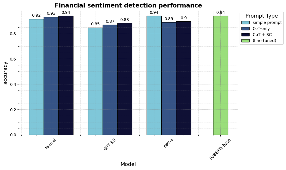
How does the standard of synthetic data compare between Mistral’s open-source Mixtral-8x7B-Instruct-v0.1 and OpenAI’s GPT3.5 and GPT4? We ran the similar pipeline and prompts explained above with gpt-3.5-turbo-0613 and gpt-4-0125-preview and reported the leads to the table below. We see that Mixtral performs higher than GPT3.5 and is on par with GPT4 for this task, depending on the prompt type. (We don’t display the outcomes for the newer gpt-3.5-turbo-0125 here because, for some reason, the performance with this model was worse than with the older default gpt-3.5-turbo-0613).

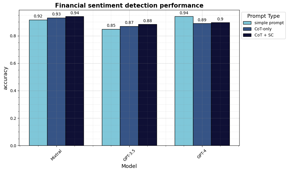
Note that this doesn’t mean Mixtral is at all times higher than GPT3.5 and on par with GPT4. GPT4 performs higher on several benchmarks. The foremost message is that open-source models can now create high-quality synthetic data.

3.3 Understand and validate your (synthetic) data

What does all this mean in practice? To date, the result’s just data annotated by some black box LLM. We could also only calculate metrics because we’ve expert annotated reference data from our example dataset. How can we trust the LLM annotations if we shouldn’t have expert annotations in a real-world scenario?

In practice, whatever annotator you employ (human annotators or LLMs), you’ll be able to only trust data you’ve validated yourself. Instructions/prompts at all times contain a level of ambiguity. Even a superbly intelligent annotator could make mistakes and must make unclear decisions when faced with often ambiguous real-world data.

Fortunately, data validation has turn out to be significantly easier over the past years with open-source tools: Argilla provides a free interface for validating and cleansing unstructured LLM outputs; LabelStudio lets you annotate data in lots of modalities; and CleanLab provides an interface for annotating and mechanically cleansing structured data; for quick and straightforward validation, it may well even be fantastic to only annotate in a straightforward Excel file.

It’s essential to spend a while annotating texts to get a feel for the information and its ambiguities. You’ll quickly learn that the model made some mistakes, but there will even be several examples where the right label is unclear and a few texts where you agree more with the choice of the LLM than with the experts who created the dataset. These mistakes and ambiguities are a standard a part of dataset creation. In truth, there are literally only only a few real-world tasks where the human expert baseline is 100% agreement. It’s an old insight recently “rediscovered” by the machine learning literature that human data is a faulty gold standard (Krippendorf 2004, Hosking et al. 2024).

After lower than an hour within the annotation interface, we gained a greater understanding of our data and corrected some mistakes. For reproducibility and to display the standard of purely synthetic data, nonetheless, we proceed using the uncleaned LLM annotations in the subsequent step.

3.3 Tune your efficient & specialized model with AutoTrain

To date, this has been an ordinary workflow of prompting an LLM through an API and validating the outputs. Now comes the extra step to enable significant resource savings: we fine-tune a smaller, more efficient, and specialized LM on the LLM’s synthetic data. This process can be called “distillation”, where the output from a bigger model (the “teacher”) is used to coach a smaller model (the “student”). While this sounds fancy, it essentially only signifies that we take our original text from the dataset and treat the predictions from the LLM as our labels for fine-tuning. If you’ve trained a classifier before, you recognize that these are the one two columns you have to train a classifier with transformers, sklearn, or another library.

We use the Hugging Face AutoTrain solution to make this process even easier. AutoTrain is a no-code interface that lets you upload a .csv file with labeled data, which the service then uses to fine-tune a model for you mechanically. This removes the necessity for coding or in-depth fine-tuning expertise for training your personal model.

On the Hugging Face website, we first click on “Spaces” at the highest after which “Create latest Space”. We then select “Docker” > “AutoTrain” and select a small A10G GPU, which costs $1.05 per hour. The Space for AutoTrain will then initialize. We will then upload our synthetic training data and expert test data via the interface and adjust the several fields, as shown within the screenshot below. Once every thing is filled in, we will click on “Start Training” and you’ll be able to follow the training process within the Space’s logs. Training a small RoBERTa-base model (~0.13 B parameters) on just 1811 data points may be very fast and mustn’t take greater than a couple of minutes. Once training is completed, the model is mechanically uploaded to your HF profile. The Space stops once training is finished, and the entire process should take at most quarter-hour and price lower than $1.

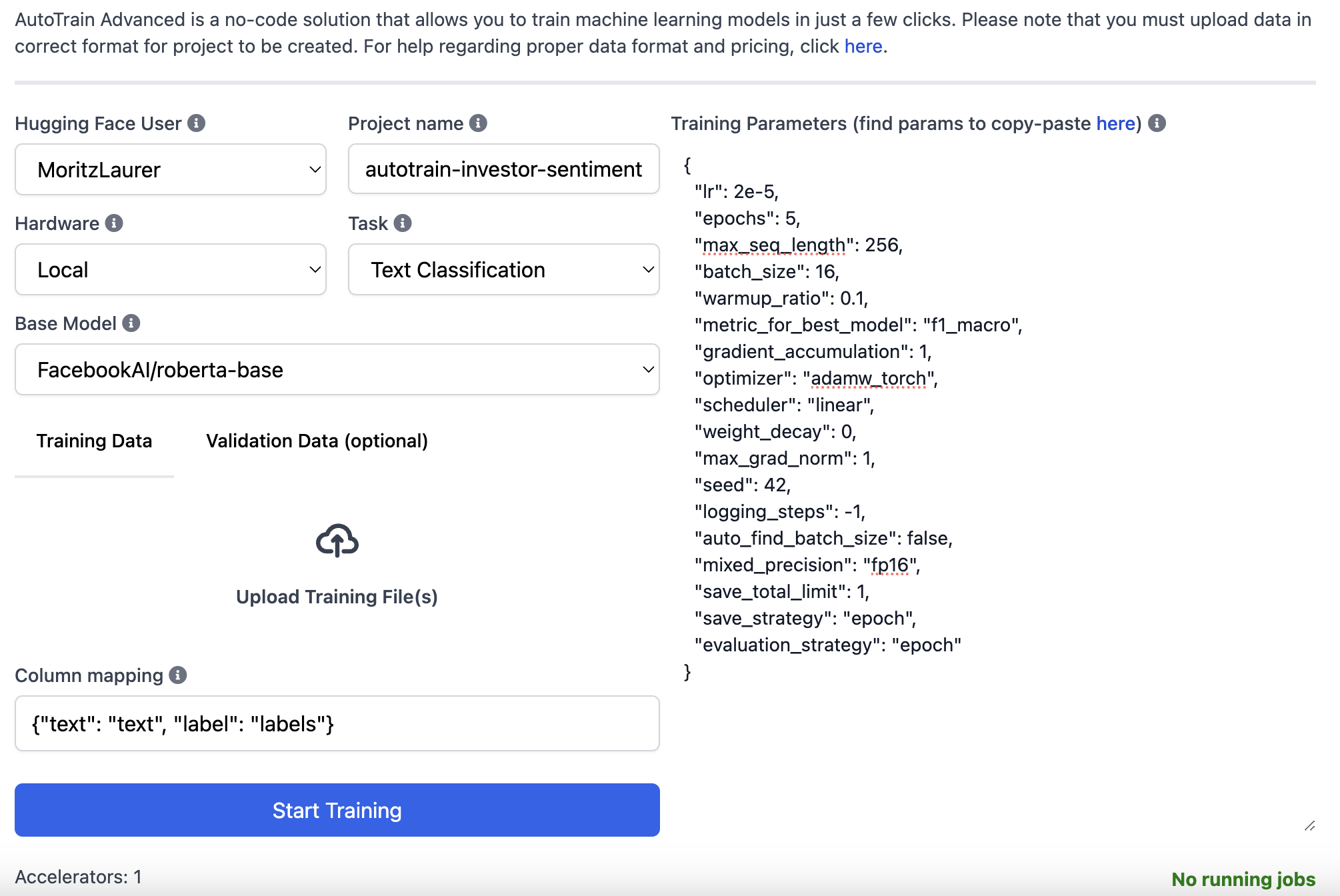
Should you want, you too can use AutoTrain entirely locally on your personal hardware, see our documentation. Advanced users can, in fact, at all times write their very own training scripts, but with these default hyperparameters, the outcomes with AutoTrain must be sufficient for a lot of classification tasks.

How well does our resulting fine-tuned ~0.13B parameter RoBERTa-base model perform in comparison with much larger LLMs? The bar chart below shows that the custom model fine-tuned on 1811 texts achieves 94% accuracy – the identical as its teacher Mixtral and GPT4! A small model could never compete with a much larger LLM out-of-the-box, but fine-tuning it on some high-quality data brings it to the identical level of performance for the duty it’s specialized in.

3.4 Pros and cons of various approaches

What are the general pros and cons of the three approaches we discussed at first: (1) manually creating your personal data and model, (2) only using an LLM API, or (3) using an LLM API to create synthetic data for a specialized model? The table below displays the trade-offs across various factors and we discuss different metrics based on our example dataset underneath.

Let’s start with task performance. As demonstrated above, the specialized model performs on par with much larger LLMs. The fine-tuned model can only do the one specific task we’ve trained it to do, but it surely does this specific task thoroughly. It will be trivial to create more training data to adapt the model to latest domains or more complex tasks. Because of synthetic data from LLMs, low performance as a result of lack of specialised data is just not an issue anymore.

Second, compute costs and inference speed. The foremost compute costs in practice can be inference, i.e. running the model after it has been trained. Let’s assume that in your production use case, you have to process 1 million sentences in a given time period. Our fine-tuned RoBERTa-base model runs efficiently on a small T4 GPU with 16GB RAM, which costs $0.6 per hour on an Inference Endpoint. It has a latency of 0.13 seconds and a throughput of 61 sentences per second with batch_size=8. This results in a complete cost of $2.7 for processing 1 million sentences.

With GPT models, we will calculate inference costs by counting tokens. Processing the tokens in 1 million sentences would cost ~$153 with GPT3.5 and ~$3061 with GPT4. The latency and throughput for these models are more complicated to calculate as they vary throughout the day depending on the present server load. Anyone working with GPT4 knows, nonetheless, that latency can often be multiple seconds and is rate-limited. Note that speed is a problem for any LLM (API), including open-source LLMs. Many generative LLMs are just too large to be fast.

Training compute costs are inclined to be less relevant, as LLMs can often be used out-of-the-box without fine-tuning, and the fine-tuning costs of smaller models are relatively small (fine-tuning RoBERTa-base costs lower than $1). Only in only a few cases do you have to spend money on pre-training a model from scratch. Training costs can turn out to be relevant when fine-tuning a bigger generative LLM to specialize it in a particular generative task.

Third, required investments in time and expertise. That is the foremost distinctiveness of LLM APIs. It’s significantly easier to send instructions to an API than to manually collect data, fine-tune a custom model, and deploy it. This is strictly where using an LLM API to create synthetic data becomes vital. Creating good training data becomes significantly easier. Superb-tuning and deployment can then be handled by services like AutoTrain and dedicated Inference Endpoints.

Fourth, control. This might be the foremost drawback of LLM APIs. By design, LLM APIs make you depending on the LLM API provider. It’s essential to send your sensitive data to another person’s servers and you can not control the reliability and speed of your system. Training your personal model enables you to select how and where to deploy it.

Lastly, environmental impact. It is very difficult to estimate the energy consumption and CO2 emissions of closed models like GPT4, given the lack of knowledge on model architecture and hardware infrastructure. The best (yet very rough) estimate we could find, puts the energy consumption per GPT4 query at around 0.0017 to 0.0026 KWh. This is able to result in very roughly 1700 – 2600 KWh for analyzing 1 million sentences. Based on the EPA CO2 equivalence calculator, that is such as 0.735 – 1.1 metric tons of CO2, or 1885 – 2883 miles driven by a mean automobile. Note that the actual CO2 emissions can vary widely depending on the energy mix within the LLM’s specific compute region. This estimate is way easier with our custom model. Analysing 1 million sentences with the custom model, takes around 4.52 hours on a T4 GPU and, on AWS servers in US East N. Virginia, this results in around 0.12 kg of CO2 (see ML CO2 Impact calculator). Running a general-purpose LLM like GPT4 with (allegedly) 8x220B parameters is ridiculously inefficient in comparison with a specialized model with ~0.13B parameters.

Conclusion

We’ve got shown the big advantages of using an LLM to create synthetic data to coach a smaller, more efficient model. While this instance only treats investor sentiment classification, the identical pipeline may very well be applied to many other tasks, from other classification tasks (e.g. customer intent detection or harmful content detection), to token classification (e.g. named entity recognition or PII detection), or generative tasks (e.g. summarization or query answering).

In 2024, it has never been easier for firms to create their very own efficient models, control their very own data and infrastructure, reduce CO2 emissions, and save compute costs and time without having to compromise on accuracy.

Now try it out yourself! Yow will discover the complete reproduction code for all numbers on this blog post, in addition to more efficient asynchronous functions with batching for API calls within the reproduction repository. We invite you to repeat and adapt our code to your use cases!