
In models, the independent variables have to be not or only barely depending on one another, i.e. that they are usually not correlated. Nevertheless, if such a dependency exists, that is known as Multicollinearity and results in unstable models and results which are difficult to interpret. The variance inflation factor is a decisive metric for recognizing multicollinearity and indicates the extent to which the correlation with other predictors increases the variance of a regression coefficient. A high value of this metric indicates a high correlation of the variable with other independent variables within the model.
In the next article, we glance intimately at multicollinearity and the VIF as a measurement tool. We also show how the VIF could be interpreted and what measures could be taken to scale back it. We also compare the indicator with other methods for measuring multicollinearity.
What’s Multicollinearity?
Multicollinearity is a phenomenon that happens in regression evaluation when two or more variables are strongly correlated with one another in order that a change in a single variable results in a change in the opposite variable. In consequence, the event of an independent variable could be predicted completely or no less than partially by one other variable. This complicates the prediction of linear regression to find out the influence of an independent variable on the dependent variable.
A distinction could be made between two sorts of multicollinearity:
- Perfect Multicollinearity: a variable is a precise linear combination of one other variable, for instance when two variables measure the identical thing in several units, equivalent to weight in kilograms and kilos.
- High Degree of Multicollinearity: Here, one variable is strongly, but not completely, explained by no less than one other variable. For instance, there may be a high correlation between an individual’s education and their income, nevertheless it will not be perfect multicollinearity.
The occurrence of multicollinearity in regressions results in serious problems as, for instance, the regression coefficients turn into unstable and react very strongly to recent data, in order that the general prediction quality suffers. Various methods could be used to acknowledge multicollinearity, equivalent to the correlation matrix or the variance inflation factor, which we are going to take a look at in additional detail in the subsequent section.
What’s the Variance Inflation Factor (VIF)?
The variance inflation factor (VIF) describes a diagnostic tool for regression models that helps to detect multicollinearity. It indicates the factor by which the variance of a coefficient increases because of the correlation with other variables. A high VIF value indicates a powerful multicollinearity of the variable with other independent variables. This negatively influences the regression coefficient estimate and ends in high standard errors. It’s due to this fact vital to calculate the VIF in order that multicollinearity is recognized at an early stage and countermeasures could be taken. :
[] [VIF = frac{1}{(1 – R^2)}]
Here (R^2) is the so-called coefficient of determination of the regression of feature (i) against all other independent variables. A high (R^2) value indicates that a big proportion of the variables could be explained by the opposite features, in order that multicollinearity is suspected.
In a regression with the three independent variables (X_1), (X_2) and (X_3), for instance, one would train a regression with (X_1) because the dependent variable and (X_2) and (X_3) as independent variables. With the assistance of this model, (R_{1}^2) could then be calculated and inserted into the formula for the VIF. This procedure would then be repeated for the remaining mixtures of the three independent variables.
A typical threshold value is VIF > 10, which indicates strong multicollinearity. In the next section, we glance in additional detail on the interpretation of the variance inflation factor.
How can different Values of the Variance Inflation Factor be interpreted?
After calculating the VIF, it will be significant to have the ability to guage what statement the worth makes in regards to the situation within the model and to have the ability to deduce whether measures are mandatory. The values could be interpreted as follows:
- VIF = 1: This value indicates that there is no such thing as a multicollinearity between the analyzed variable and the opposite variables. Which means that no further motion is required.
- VIF between 1 and 5: If the worth is within the range between 1 and 5, then there may be multicollinearity between the variables, but this will not be large enough to represent an actual problem. Quite, the dependency continues to be moderate enough that it could actually be absorbed by the model itself.
- VIF > 5: In such a case, there may be already a high degree of multicollinearity, which requires intervention in any case. The usual error of the predictor is prone to be significantly excessive, so the regression coefficient could also be unreliable. Consideration needs to be given to combining the correlated predictors into one variable.
- VIF > 10: With such a worth, the variable has serious multicollinearity and the regression model may be very prone to be unstable. On this case, consideration needs to be given to removing the variable to acquire a more powerful model.
Overall, a high VIF value indicates that the variable could also be redundant, because it is extremely correlated with other variables. In such cases, various measures needs to be taken to scale back multicollinearity.
What measures help to scale back the VIF?
There are numerous ways to avoid the results of multicollinearity and thus also reduce the variance inflation factor. The preferred measures include:
- Removing highly correlated variables: Especially with a high VIF value, removing individual variables with high multicollinearity is a very good tool. This could improve the outcomes of the regression, as redundant variables estimate the coefficients more unstable.
- Principal component evaluation (PCA): The core idea of principal component evaluation is that several variables in a knowledge set may measure the identical thing, i.e. be correlated. Which means that the assorted dimensions could be combined into fewer so-called principal components without compromising the importance of the information set. Height, for instance, is extremely correlated with shoe size, as tall people often have taller shoes and vice versa. Which means that the correlated variables are then combined into uncorrelated foremost components, which reduces multicollinearity without losing vital information. Nevertheless, this can also be accompanied by a lack of interpretability, because the principal components don’t represent real characteristics, but a mixture of various variables.
- Regularization Methods: Regularization comprises various methods which are utilized in statistics and machine learning to manage the complexity of a model. It helps to react robustly to recent and unseen data and thus enables the generalizability of the model. That is achieved by adding a penalty term to the model’s optimization function to stop the model from adapting an excessive amount of to the training data. This approach reduces the influence of highly correlated variables and lowers the VIF. At the identical time, nevertheless, the accuracy of the model will not be affected.
These methods could be used to effectively reduce the VIF and combat multicollinearity in a regression. This makes the outcomes of the model more stable and the usual error could be higher controlled.
How does the VIF compare to other methods?
The variance inflation factor is a widely used technique to measure multicollinearity in a knowledge set. Nevertheless, other methods can offer specific benefits and drawbacks in comparison with the VIF, depending on the appliance.
Correlation Matrix
The correlation matrix is a statistical method for quantifying and comparing the relationships between different variables in a knowledge set. The pairwise correlations between all mixtures of two variables are shown in a tabular structure. Each cell within the matrix incorporates the so-called correlation coefficient between the 2 variables defined within the column and the row.
This value could be between -1 and 1 and provides information on how the 2 variables relate to one another. A positive value indicates a positive correlation, meaning that a rise in a single variable results in a rise in the opposite variable. The precise value of the correlation coefficient provides information on how strongly the variables move about one another. With a negative correlation coefficient, the variables move in opposite directions, meaning that a rise in a single variable results in a decrease in the opposite variable. Finally, a coefficient of 0 indicates that there is no such thing as a correlation.
A correlation matrix due to this fact fulfills the aim of presenting the correlations in a knowledge set in a fast and easy-to-understand way and thus forms the premise for subsequent steps, equivalent to model selection. This makes it possible, for instance, to acknowledge multicollinearity, which may cause problems with regression models, because the parameters to be learned are distorted.
In comparison with the VIF, the correlation matrix only offers a surface evaluation of the correlations between variables. Nevertheless, the most important difference is that the correlation matrix only shows the pairwise comparisons between variables and never the simultaneous effects between several variables. As well as, the VIF is more useful for quantifying exactly how much multicollinearity affects the estimate of the coefficients.
Eigenvalue Decomposition
Eigenvalue decomposition is a technique that builds on the correlation matrix and mathematically helps to discover multicollinearity. Either the correlation matrix or the covariance matrix could be used. On the whole, small eigenvalues indicate a stronger, linear dependency between the variables and are due to this fact an indication of multicollinearity.
In comparison with the VIF, the eigenvalue decomposition offers a deeper mathematical evaluation and may in some cases also help to detect multicollinearity that will have remained hidden by the VIF. Nevertheless, this method is way more complex and difficult to interpret.
The VIF is an easy and easy-to-understand method for detecting multicollinearity. In comparison with other methods, it performs well since it allows a precise and direct evaluation that’s at the extent of the person variables.
The right way to detect Multicollinearity in Python?
Recognizing multicollinearity is a vital step in data preprocessing in machine learning to coach a model that’s as meaningful and robust as possible. On this section, we due to this fact take a better take a look at how the VIF could be calculated in Python and the way the correlation matrix is created.
Calculating the Variance Inflation Think about Python
The Variance Inflation Factor could be easily used and imported in Python via the statsmodels library. Assuming we have already got a Pandas DataFrame in a variable X that incorporates the independent variables, we are able to simply create a brand new, empty DataFrame for calculating the VIFs. The variable names and values are then saved on this frame.
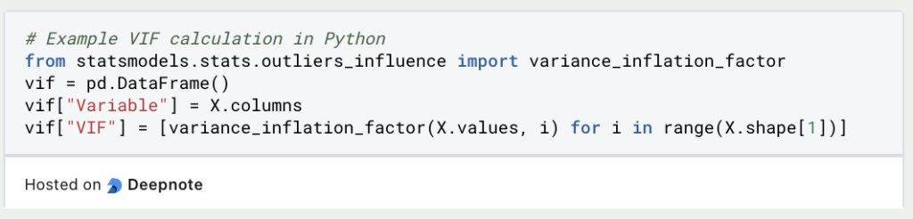
A brand new row is created for every independent variable in X within the Variable column. It’s then iterated through all variables in the information set and the variance inflation factor is calculated for the values of the variables and again saved in a listing. This list is then stored as column VIF within the DataFrame.
Calculating the Correlation Matrix
In Python, a correlation matrix could be easily calculated using Pandas after which visualized as a heatmap using Seaborn. For instance this, we generate random data using NumPy and store it in a DataFrame. As soon as the information is stored in a DataFrame, the correlation matrix could be created using the corr() function.
If no parameters are defined throughout the function, the Pearson coefficient is utilized by default to calculate the correlation matrix. Otherwise, you may also define a distinct correlation coefficient using the tactic parameter.

Finally, the heatmap is visualized using seaborn. To do that, the heatmap() function is named and the correlation matrix is passed. Amongst other things, the parameters could be used to find out whether the labels needs to be added and the colour palette could be specified. The diagram is then displayed with the assistance of matplolib.
That is what it’s best to take with you
- The variance inflation factor is a key indicator for recognizing multicollinearity in a regression model.
- The coefficient of determination of the independent variables is used for the calculation. Not only the correlation between two variables could be measured, but additionally mixtures of variables.
- On the whole, a response needs to be taken if the VIF is bigger than five, and appropriate measures needs to be introduced. For instance, the affected variables could be faraway from the information set or the principal component evaluation could be performed.
- In Python, the VIF could be calculated directly using statsmodels. To do that, the information have to be stored in a DataFrame. The correlation matrix can be calculated using Seaborn to detect multicollinearity.